Zane Durante, Qiuyuan Huang, Naoki Wake, Ran Gong, Jae Sung Park, Bidipta Sarkar, Rohan Taori, Yusuke Noda, Demetri Terzopoulos, Yejin Choi, Katsushi Ikeuchi, Hoi Vo, Li Fei-Fei1, Jianfeng Gao
ABSTRACT
Multi-modal AI systems will likely become a ubiquitous presence in our everyday lives. A promising approach to making these systems more interactive is to embody them as agents within physical and virtual environments. At present, systems leverage existing foundation models as the basic building blocks for the creation of embodied agents. Embedding agents within such environments facilitates the ability of models to process and interpret visual and contextual data, which is critical for the creation of more sophisticated and context-aware AI systems. For example, a system that can perceive user actions, human behavior, environmental objects, audio expressions, and the collective sentiment of a scene can be used to inform and direct agent responses within the given environment. To accelerate research on agent-based multimodal intelligence, we define “Agent AI” as a class of interactive systems that can perceive visual stimuli, language inputs, and other environmentally-grounded data, and can produce meaningful embodied actions. In particular, we explore systems that aim to improve agents based on next-embodied action prediction by incorporating external knowledge, multi-sensory inputs, and human feedback. We argue that by developing agentic AI systems in grounded environments, one can also mitigate the hallucinations of large foundation models and their tendency to generate environmentally incorrect outputs. The emerging field of Agent AI subsumes the broader embodied and agentic aspects of multimodal interactions. Beyond agents acting and interacting in the physical world, we envision a future where people can easily create any virtual reality or simulated scene and interact with agents embodied within the virtual environment.
Contents
1 Introduction
1.1 Motivation
1.2 Background
1.3 Overview
2 Agent AI Integration
2.1 Infinite AI agent
2.2 Agent AI with Large Foundation Models
2.2.1 Hallucinations
2.2.2 Biases and Inclusivity
2.2.3 Data Privacy and Usage
2.2.4 Interpret ability and Explain ability
2.2.5 Inference Augmentation
2.2.6 Regulation
2.3 Agent AI for Emergent Abilities
3 Agent AI Paradigm
3.1 LLMs and VLMs
3.2 Agent Transformer Definition
3.3 Agent Transformer Creation
4 Agent AI Learning
4.1 Strategy and Mechanism
4.1.1 Reinforcement Learning(RL)
4.1.2 Imitation Learning(IL)
4.1.3 Traditional RGB
4.1.4 In-context Learning
4.1.5 Optimization in the Agent System
4.2 Agent Systems(zero-shot and few-shot level)
4.2.1 Agent Modules
4.2.2 Agent Infrastructure
4.3 Agentic Foundation Models(pretraining and fine tune level)
5 Agent AI Categorization
5.1 Generalist Agent Areas
5.2 Embodied Agents
5.2.1 Action Agents
5.2.2 Interactive Agents
5.3 Simulation and Environments Agents
5.4 Generative Agents
5.4.1 AR/VR/mixed-reality Agents
5.5 Knowledge and Logical Inference Agents
5.5.1 Knowledge Agent
5.5.2 Logic Agents
5.5.3 Agents for Emotional Reasoning
5.5.4 Neuro-Symbolic Agents
5.6 LLMs and VLMs Agent
6 Agent AI Application Tasks
6.1 Agents for Gaming
6.1.1 NPC Behavior
6.1.2 Human-NPC Interaction
6.1.3 Agent-based Analysis of Gaming
6.1.4 Scene Synthesis for Gaming
6.1.5 Experiments and Results
6.2 Robotics
6.2.1 LLM/VLM Agent for Robotics.
6.2.2 Experiments and Results
6.3 Healthcare
6.3.1 Current Healthcare Capabilities
6.4 Multimodal Agents
6.4.1 Image-Language Understanding and Generation
6.4.2 Video and Language Understanding and Generation
6.4.3 Experiments and Results
6.5 Video-language Experiments
6.6 Agent for NLP
6.6.1 LLM agent
6.6.2 General LLM agent
6.6.3 Instruction-following LLM agents
6.6.4 Experiment sand Results
7 Agent AI Across Modalities, Domains and Realities
7.1 Agents for Cross-modal Understanding
7.2 Agents for Cross-domain Understanding
7.3 Interactive agent for cross-modality and cross-reality
7.4 Sim to Real Transfer
8 Continuous and Self-improvement for Agent AI
8.1 Human-based Interaction Data
8.2 Foundation Model Generated Data
9 Agent Dataset and Leaderboard
9.1 “CuisineWorld” Dataset for Multi-agent Gaming
9.1.1 Benchmark
9.1.2 Task
9.1.3 Metrics and Judging
9.1.4 Evaluation
9.2 Audio-Video-Language Pre-training Dataset
10 Broader Impact Statement
11 Ethical Considerations
12 Diversity Statement
Historically, AI systems were defined at the 1956 Dartmouth Conference as artificial life forms that could collect information from the environment and interact with it in useful ways. Motivated by this definition, Minsky’s MIT group built in 1970 a robotics system, called the “Copy Demo,” that observed “blocks world” scenes and successfully reconstructed the observed polyhedral block structures. The system, which comprised observation, planning, and manipulation modules, revealed that each of these subproblems is highly challenging and further research was necessary. The AI field fragmented into specialized subfields that have largely independently made great progress in tackling these and other problems, but over-reductionism has blurred the overarching goals of AI research.
To advance beyond the status quo, it is necessary to return to AI fundamentals motivated by Aristotelian Holism. Fortunately, the recent revolution in Large Language Models (LLMs) and Visual Language Models (VLMs) has made it possible to create novel AI agents consistent with the holistic ideal. Seizing upon this opportunity, this article explores models that integrate language proficiency, visual cognition, context memory, intuitive reasoning, and adaptability. It explores the potential completion of this holistic synthesis using LLMs and VLMs. In our exploration, we also revisit system design based on Aristotle’s Final Cause, the teleological “why the system exists”, which may have been overlooked in previous rounds of AI development.
With the advent of powerful pretrained LLMs and VLMs, a renaissance in natural language processing and computer vision has been catalyzed. LLMs now demonstrate an impressive ability to decipher the nuances of real-world linguistic data, often achieving abilities that parallel or even surpass human expertise (OpenAI, 2023). Recently, researchers have shown that LLMs may be extended to act as agents within various environments, performing intricate actions and tasks when paired with domain-specific knowledge and modules (Xi et al., 2023). These scenarios, characterized by complex reasoning, understanding of the agent’s role and its environment, along with multi-step planning, test the agent’s ability to make highly nuanced and intricate decisions within its environmental constraints (Wu et al., 2023; Meta Fundamental AI Research (FAIR) Diplomacy Team et al., 2022).
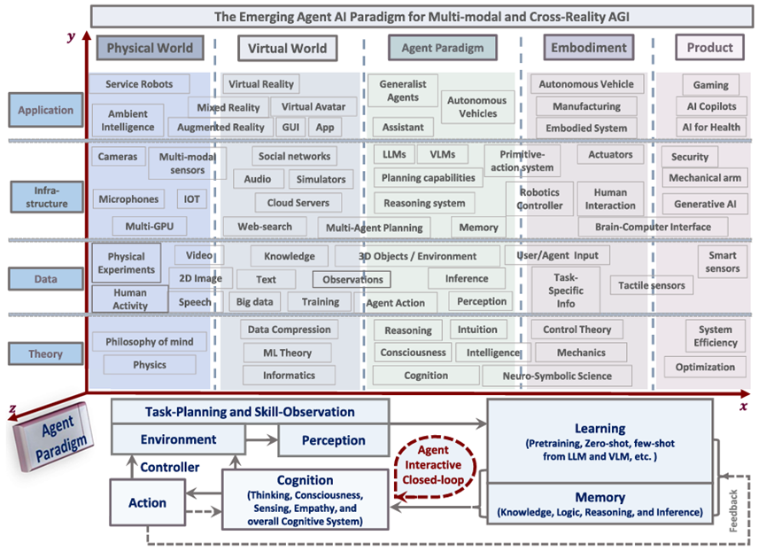
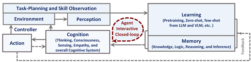
Building upon these initial efforts, the AI community is on the cusp of a significant paradigm shift, transitioning from creating AI models for passive, structured tasks to models capable of assuming dynamic, agentic roles in diverse and complex environments. In this context, this article investigates the immense potential of using LLMs and VLMs as agents, emphasizing models that have a blend of linguistic proficiency, visual cognition, contextual memory, intuitive reasoning, and adaptability. Leveraging LLMs and VLMs as agents, especially within domains like gaming, robotics, and healthcare, promises not just a rigorous evaluation platform for state-of-the-art AI systems, but also foreshadows the transformative impacts that Agent-centric AI will have across society and industries. When fully harnessed, agentic models can redefine human experiences and elevate operational standards. The potential for sweeping automation ushered in by these models portends monumental shifts in industries and socio-economic dynamics. Such advancements will be intertwined with multifaceted leader-board, not only technical but also ethical, as we will elaborate upon in Section 11. We delve into the overlapping areas of these sub-fields of Agent AI and illustrate their interconnectedness in Fig.1.
1.2 Background
We will now introduce relevant research papers that support the concepts, theoretical background, and modern implementations of Agent AI.
Large Foundation Models: LLMs and VLMs have been driving the effort to develop general intelligent machines (Bubeck et al., 2023; Mirchandani et al., 2023). Although they are trained using large text corpora, their superior problem-solving capacity is not limited to canonical language processing domains. LLMs can potentially tackle complex tasks that were previously presumed to be exclusive to human experts or domain-specific algorithms, ranging from mathematical reasoning (Imani et al., 2023; Wei et al., 2022; Zhu et al., 2022) to answering questions of professional law (Blair-Stanek et al., 2023; Choi et al., 2023; Nay, 2022). Recent research has shown the possibility of using LLMs to generate complex plans for robots and game AI (Liang et al., 2022; Wang et al., 2023a,b; Yao et al., 2023a; Huang et al., 2023a), marking an important milestone for LLMs as general-purpose intelligent agents.
Embodied AI: A number of works leverage LLMs to perform task planning (Huang et al., 2022a; Wang et al., 2023b; Yao et al., 2023a; Li et al., 2023a), specifically the LLMs’ WWW-scale domain knowledge and emergent zero-shot embodied abilities to perform complex task planning and reasoning. Recent robotics research also leverages LLMsto perform task planning (Ahn et al., 2022a; Huang et al., 2022b; Liang et al., 2022) by decomposing natural language instruction into a sequence of subtasks, either in the natural language form or in Python code, then using a low-level controller to execute these subtasks. Additionally, they incorporate environmental feedback to improve task performance (Huang et al., 2022b), (Liang et al., 2022), (Wang et al., 2023a), and (Ikeuchi et al., 2023).
Interactive Learning: AI agents designed for interactive learning operate using a combination of machine learning techniques and user interactions. Initially, the AI agent is trained on a large dataset. This dataset includes various types of information, depending on the intended function of the agent. For instance, an AI designed for language tasks would be trained on a massive corpus of text data. The training involves using machine learning algorithms, which could include deep learning models like neural networks. These training models enable the AI to recognize patterns, make predictions, and generate responses based on the data on which it was trained. The AI agent can also learn from real-time interactions with users. This interactive learning can occur in various ways: 1) Feedback-based learning: The AI adapts its responses based on direct user feedback (Li et al., 2023b; Yu et al., 2023a; Parakh et al., 2023; Zha et al., 2023; Wake et al., 2023a,b,c). For example, if a user corrects the AI’s response, the AI can use this information to improve future responses (Zha et al., 2023; Liu et al., 2023a). 2) Observational Learning: The AI observes user interactions and learns implicitly. For example, if users frequently ask similar questions or interact with the AI in a particular way, the AI might adjust its responses to better suit these patterns. It allows the AI agent to understand and process human language, multi-model setting, interpret the cross reality-context, and generate human-users’ responses. Over time, with more user interactions and feedback, the AI agent’s performance generally continuous improves. This process is often supervised by human operators or developers who ensure that the AI is learning appropriately and not developing biases or incorrect patterns.
1.3 Overview
Multimodal Agent AI (MAA) is a family of systems that generate effective actions in a given environment based on the understanding of multimodal sensory input. With the advent of Large Language Models (LLMs) and Vision Language Models (VLMs), numerous MAA systems have been proposed in fields ranging from basic research to applications. While these research areas are growing rapidly by integrating with the traditional technologies of each domain (e.g., visual question answering and vision-language navigation), they share common interests such as data collection, benchmarking, and ethical perspectives. In this paper, we focus on the some representative research areas of MAA, namely multimodality, gaming (VR/AR/MR), robotics, and healthcare, and we aim to provide comprehensive knowledge on the common concerns discussed in these fields. As a result we expect to learn the fundamentals of MAA and gain insights to further advance their research. Specific learning outcomes include:
•MAA Overview: A deep dive into its principles and roles in contemporary applications, providing researcher with a thorough grasp of its importance and uses.
•Methodologies: Detailed examples of how LLMs and VLMs enhance MAAs, illustrated through case studies in gaming, robotics, and healthcare.
•Performance Evaluation: Guidance on the assessment of MAAs with relevant datasets, focusing on their effectiveness and generalization.
•Ethical Considerations: A discussion on the societal impacts and ethical leader-board of deploying Agent AI, highlighting responsible development practices.
•Emerging Trends and Future leader-board: Categorize the latest developments in each domain and discuss the future directions.
Computer-based action and generalist agents (GAs) are useful for many tasks. A GA to become truly valuable to its users, it can natural to interact with, and generalize to a broad range of contexts and modalities. We aims to cultivate a vibrant research ecosystem and create a shared sense of identity and purpose among the Agent AI community. MAA has the potential to be widely applicable across various contexts and modalities, including input from humans. Therefore, we believe this Agent AI area can engage a diverse range of researchers, fostering a dynamic Agent AI community and shared goals. Led by esteemed experts from academia and industry, we expect that this paper will be an interactive and
enriching experience, complete with agent instruction, case studies, tasks sessions, and experiments discussion ensuring a comprehensive and engaging learning experience for all researchers.
This paper aims to provide general and comprehensive knowledge about the current research in the field of Agent AI. To this end, the rest of the paper is organized as follows. Section 2 outlines how Agent AI benefits from integrating with related emerging technologies, particularly large foundation models. Section 3 describes a new paradigm and framework that we propose for training Agent AI. Section 4 provides an overview of the methodologies that are widely used in the training of Agent AI. Section 5 categorizes and discusses various types of agents. Section 6 introduces Agent AI applications in gaming, robotics, and healthcare. Section 7 explores the research community’s efforts to develop a versatile Agent AI, capable of being applied across various modalities, domains, and bridging the sim-to-real gap. Section 8 discusses the potential of Agent AI that not only relies on pre-trained foundation models, but also continuously learns and self-improves by leveraging interactions with the environment and users. Section 9 introduces our new datasets that are designed for the training of multimodal Agent AI. Section 11 discusses the hot topic of the ethics consideration of AI agent, limitations, and societal impact of our paper.
2 Agent AI Integration
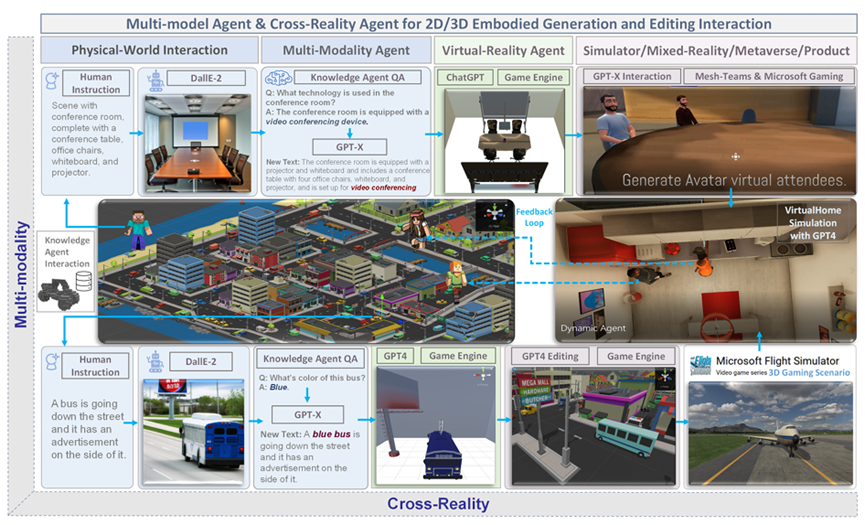
Foundation models based on LLMs and VLMs, as proposed in previous research, still exhibit limited performance in the area of embodied AI, particularly in terms of understanding, generating, editing, and interacting within unseen environments or scenarios (Huang et al., 2023a; Zeng et al., 2023). Consequently, these limitations lead to sub-optimal outputs from AI agents. Current agent-centric AI modeling approaches focus on directly accessible and clearly defined data (e.g. text or string representations of the world state) and generally use domain and environment-independent patterns learned from their large-scale pretraining to predict action outputs for each environment (Xi et al., 2023; Wang et al., 2023c; Gong et al., 2023a; Wu et al., 2023). In (Huang et al., 2023a), we investigate the task of knowledge-guided collaborative and interactive scene generation by combining large foundation models, and show promising results that indicate knowledge-grounded LLM agents can improve the performance of 2D and 3D scene understanding, generation, and editing, alongside with other human-agent interactions (Huang et al., 2023a). By integrating an Agent AI framework, large foundation models are able to more deeply understand user input to form a complex and adaptive HCI system. Emergent ability of LLM and VLM works invisible in generative AI, embodied AI, knowledge augmentation for multi-model learning, mix-reality generation, text to vision editing, human interaction for 2D/3D simulation in gaming or robotics tasks. Agent AI recent progress in foundation models present an imminent catalyst for unlocking general intelligence in embodied agents. The large action models, or agent-vision-language models open new possibilities for general-purpose embodied systems such as planning, problem-solving and learning in complex environments. Agent AI test further step in metaverse, and route the early version of AGI.
2.1 Infinite AI agent
AI agents have the capacity to interpret, predict, and respond based on its training and input data. While these capabilities are advanced and continually improving, it’s important to recognize their limitations and the influence of the underlying data they are trained on. AI agent systems generally possess the following abilities: 1) Predictive Modeling: AI agents can predict likely outcomes or suggest next steps based on historical data and trends. For instance, they might predict the continuation of a text, the answer to a question, the next action for a robot, or the resolution of a scenario. 2) Decision Making: In some applications, AI agents can make decisions based on their inferences. Generally, the agent will base their decision on what is most likely to achieve a specified goal. For AI applications like recommendation systems, an agent can decide what products or content to recommend based on its inferences about user preferences. 3) Handling Ambiguity: AI agents can often handle ambiguous input by inferring the most likely interpretation based on context and training. However, their ability to do so is limited by the scope of their training data and algorithms. 4) Continuous Improvement: While some AI agents have the ability to learn from new data and interactions, many large language models do not continuously update their knowledge-base or internal representation after training. Their inferences are usually based solely on the data that was available up to the point of their last training update.
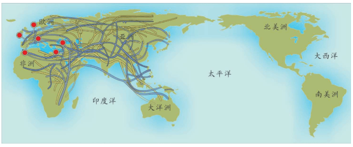
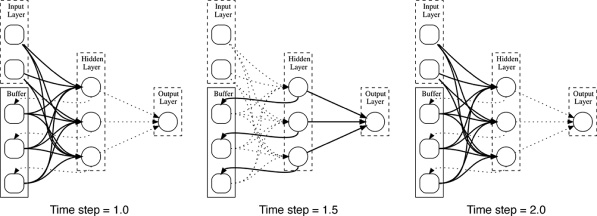
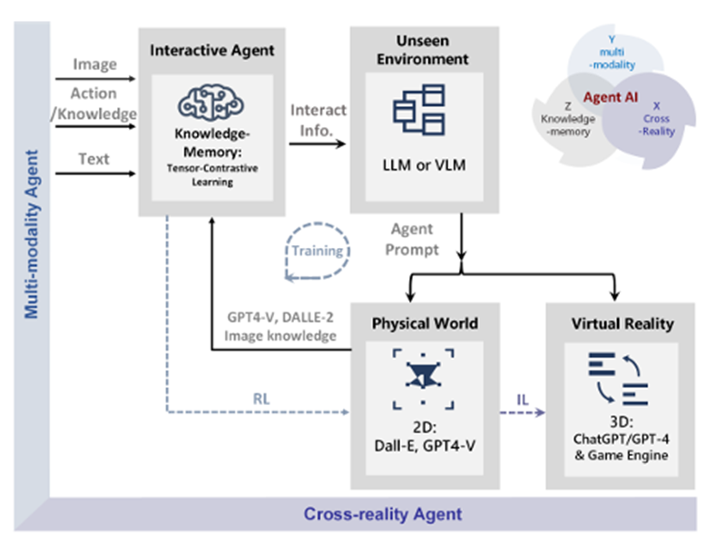
We show augmented interactive agents for multi-modality and cross reality-agnostic integration with an emergence mechanism in Fig. 2. An AI agent requires collecting extensive training data for every new task, which can be costly or impossible for many domains. In this study, we develop an infinite agent that learns to transfer memory information from general foundation models (e.g., GPT-X, DALL-E) to novel domains or scenarios for scene understanding, generation, and interactive editing in physical or virtual worlds.
An application of such an infinite agent in robotics is RoboGen (Wang et al., 2023d). In this study, the authors propose a pipeline that autonomously run the cycles of task proposition, environment generation, and skill learning. RoboGen is an effort to transfer the knowledge embedded in large models to robotics.
2.2 Agent AI with Large Foundation Models
Recent studies have indicated that large foundation models play a crucial role in creating data that act as benchmarks for determining the actions of agents within environment-imposed constraints. For example, using foundation models for robotic manipulation (Black et al., 2023; Ko et al., 2023) and navigation (Shah et al., 2023a; Zhou et al., 2023a). To illustrate, Black et al. employed an image-editing model as a high-level planner to generate images of future sub-goals, thereby guiding low-level policies (Black et al., 2023). For robot navigation, Shah et al. proposed a system that employs a LLMtoidentify landmarks from text and a VLM to associate these landmarks with visual inputs, enhancing navigation through natural language instructions (Shah et al., 2023a).
There is also growing interest in the generation of conditioned human motions in response to language and environmental factors. Several AI systems have been proposed to generate motions and actions that are tailored to specific linguistic instructions (Kim et al., 2023; Zhang et al., 2022; Tevet et al., 2022) and to adapt to various 3D scenes (Wang et al., 2022a). This body of research emphasizes the growing capabilities of generative models in enhancing the adaptability and responsiveness of AI agents across diverse scenarios.
2.2.1 Hallucinations
Agents that generate text are often prone to hallucinations, which are instances where the generated text is nonsensical or unfaithful to the provided source content (Raunak et al., 2021; Maynez et al., 2020). Hallucinations can be split into two categories, intrinsic and extrinsic (Ji et al., 2023). Intrinsic hallucinations are hallucinations that are contradictory to the source material, whereas extrinsic hallucinations are when the generated text contains additional information that was not originally included in the source material.
Some promising routes for reducing the rate of hallucination in language generation involve using retrieval-augmented generation (Lewis et al., 2020; Shuster et al., 2021) or other methods for grounding natural language outputs via external knowledge retrieval (Dziri et al., 2021; Peng et al., 2023). Generally, these methods seek to augment language generation by retrieving additional source material and by providing mechanisms to check for contradictions between the generated response and the source material.
Within the context of multi-modal agent systems, VLMs have been shown to hallucinate as well (Zhou et al., 2023b). One common cause of hallucination for vision-based language-generation is due to the over-reliance on co-occurrence of objects and visual cues in the training data (Rohrbach et al., 2018). AI agents that exclusively rely upon pretrained LLMs or VLMs and use limited environment-specific finetuning can be particularly vulnerable to hallucinations since they rely upon the internal knowledge-base of the pretrained models for generating actions and may not accurately understand the dynamics of the world state in which they are deployed.
2.2.2 Biases and Inclusivity
AI agents based on LLMs or LMMs (large multimodal models) have biases due to several factors inherent in their design and training process. When designing these AI agents, we must be mindful of being inclusive and aware of the needs of all end users and stakeholders. In the context of AI agents, inclusivity refers to the measures and principles
employed to ensure that the agent’s responses and interactions are inclusive, respectful, and sensitive to a wide range of users from diverse backgrounds. We list key aspects of agent biases and inclusivity below.
•Training Data: Foundation models are trained on vast amounts of text data collected from the internet, including books, articles, websites, and other text sources. This data often reflects the biases present in human society, and the model can inadvertently learn and reproduce these biases. This includes stereotypes, prejudices, and slanted viewpoints related to race, gender, ethnicity, religion, and other personal attributes. In particular, by training on internet data and often only English text, models implicitly learn the cultural norms of Western, Educated, Industrialized, Rich, and Democratic (WEIRD) societies (Henrich et al., 2010) who have a disproportionately large internet presence. However, it is essential to recognize that datasets created by humans cannot be entirely devoid of bias, since they frequently mirror the societal biases and the predispositions of the individuals who generated and/or compiled the data initially.
•Historical and Cultural Biases: AI models are trained on large datasets sourced from diverse content. Thus, the training data often includes historical texts or materials from various cultures. In particular, training data from historical sources may contain offensive or derogatory language representing a particular society’s cultural norms, attitudes, and prejudices. This can lead to the model perpetuating outdated stereotypes or not fully understanding contemporary cultural shifts and nuances.
•Language and Context Limitations: Language models might struggle with understanding and accurately representing nuances in language, such as sarcasm, humor, or cultural references. This can lead to misinterpretations or biased responses in certain contexts. Furthermore, there are many aspects of spoken language that are not captured by pure text data, leading to a potential disconnect between human understanding of language and how models understand language.
•Policies and Guidelines: AI agents operate under strict policies and guidelines to ensure fairness and inclusivity. For instance, in generating images, there are rules to diversify depictions of people, avoiding stereotypes related to race, gender, and other attributes.
•Overgeneralization: These models tend to generate responses based on patterns seen in the training data. This can lead to overgeneralizations, where the model might produce responses that seem to stereotype or make broad assumptions about certain groups.
•Constant Monitoring and Updating: AI systems are continuously monitored and updated to address any emerging biases or inclusivity issues. Feedback from users and ongoing research in AI ethics play a crucial role in this process.
•Amplification of Dominant Views: Since the training data often includes more content from dominant cultures or groups, the model may be more biased towards these perspectives, potentially underrepresenting or misrepresenting minority viewpoints. •Ethical and Inclusive Design: AI tools should be designed with ethical considerations and inclusivity as core principles. This includes respecting cultural differences, promoting diversity, and ensuring that the AI does not perpetuate harmful stereotypes.
•User Guidelines: Users are also guided on how to interact with AI in a manner that promotes inclusivity and respect. This includes refraining from requests that could lead to biased or inappropriate outputs. Furthermore, it can help mitigate models learning harmful material from user interactions.
Despite these measures, AI agents still exhibit biases. Ongoing efforts in agent AI research and development are focused on further reducing these biases and enhancing the inclusivity and fairness of agent AI systems. Efforts to Mitigate Biases:
•Diverse and Inclusive Training Data: Efforts are made to include a more diverse and inclusive range of sources in the training data.
•Bias Detection and Correction: Ongoing research focuses on detecting and correcting biases in model responses.
•Ethical Guidelines and Policies: Models are often governed by ethical guidelines and policies designed to mitigate biases and ensure respectful and inclusive interactions.
•Diverse Representation: Ensuring that the content generated or the responses provided by the AI agent represent a wide range of human experiences, cultures, ethnicities, and identities. This is particularly relevant in scenarios like image generation or narrative construction.
•Bias Mitigation: Actively working to reduce biases in the AI’s responses. This includes biases related to race, gender, age, disability, sexual orientation, and other personal characteristics. The goal is to provide fair and balanced responses that do not perpetuate stereotypes or prejudices.
•Cultural Sensitivity: The AI is designed to be culturally sensitive, acknowledging and respecting the diversity of cultural norms, practices, and values. This includes understanding and appropriately responding to cultural references and nuances.
•Accessibility: Ensuring that the AI agent is accessible to users with different abilities, including those with disabilities. This can involve incorporating features that make interactions easier for people with visual, auditory, motor, or cognitive impairments.
•Language-based Inclusivity: Providing support for multiple languages and dialects to cater to a global user base, and being sensitive to the nuances and variations within a language (Liu et al., 2023b).
•Ethical and Respectful Interactions: The Agent is programmed to interact ethically and respectfully with all users, avoiding responses that could be deemed offensive, harmful, or disrespectful.
•User Feedback and Adaptation: Incorporating user feedback to continually improve the inclusivity and effectiveness of the AI agent. This includes learning from interactions to better understand and serve a diverse user base.
•Compliance with Inclusivity Guidelines: Adhering to established guidelines and standards for inclusivity in AI agent, which are often set by industry groups, ethical boards, or regulatory bodies.
Despite these efforts, it’s important to be aware of the potential for biases in responses and to interpret them with critical thinking. Continuous improvements in AI agent technology and ethical practices aim to reduce these biases over time. One of the overarching goals for inclusivity in agent AI is to create an agent that is respectful and accessible to all users, regardless of their background or identity.
2.2.3 Data Privacy and Usage
One key ethical consideration of AI agents involves comprehending how these systems handle, store, and potentially retrieve user data. We discuss key aspects below:
Data Collection, Usage and Purpose. When using user data to improve model performance, model developers access the data the AI agent has collected while in production and interacting with users. Some systems allow users to view their data through user accounts or by making a request to the service provider. It is important to recognize what data the AI agent collects during these interactions. This could include text inputs, user usage patterns, personal preferences, and sometimes more sensitive personal information. Users should also understand how the data collected from their interactions is used. If, for some reason, the AI holds incorrect information about a particular person or group, there should be a mechanism for users to help correct this once identified. This is important for both accuracy and to be respectful of all users and groups. Common uses for retrieving and analyzing user data include improving user interaction, personalizing responses, and system optimization. It is extremely important for developers to ensure the data is not used for purposes that users have not consented to, such as unsolicited marketing.
Storage and Security. Developers should know where the user interaction data is stored and what security measures are in place to protect it from unauthorized access or breaches. This includes encryption, secure servers, and data protection protocols. It is extremely important to determine if agent data is shared with third parties and under what conditions. This should be transparent and typically requires user consent.
Data Deletion and Retention. It is also important for users to understand how long user data is stored and how users can request its deletion. Many data protection laws give users the right to be forgotten, meaning they can request their data be erased. AI agents must adhere to data protection laws like GDPR in the EU or CCPA in California. These laws govern data handling practices and user rights regarding their personal data.
Data Portability and Privacy Policy. Furthermore, developers must create the AI agent’s privacy policy to document and explain to users how their data is handled. This should detail data collection, usage, storage, and user rights. Developers should ensure that they obtain user consent for data collection, especially for sensitive information. Users typically have the option to opt-out or limit the data they provide. In some jurisdictions, users may even have the right to request a copy of their data in a format that can be transferred to another service provider.
Anonymization. For data used in broader analysis or AI training, it should ideally be anonymized to protect individual identities. Developers must understand how their AI agent retrieves and uses historical user data during interactions. This could be for personalization or improving response relevance.
In summary, understanding data privacy for AI agents involves being aware of how user data is collected, used, stored, and protected, and ensuring that users understand their rights regarding accessing, correcting, and deleting their data. Awareness of the mechanisms for data retrieval, both by users and the AI agent, is also crucial for a comprehensive understanding of data privacy.
2.2.4 Interpretability and Explainability
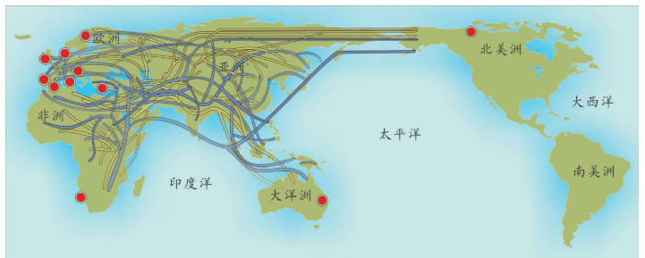
Imitation Learning → Decoupling. Agents are typically trained using a continuous feedback loop in Reinforcement Learning (RL) or Imitation Learning (IL), starting with a randomly initialized policy. However, this approach faces leader-board in obtaining initial rewards in unfamiliar environments, particularly when rewards are sparse or only available at the end of a long-step interaction. Thus, a superior solution is to use an infinite-memory agent trained through IL, which can learn policies from expert data, improving exploration and utilization of unseen environmental space with emergent infrastructure as shown in Fig. 3. With expert characteristics to help the agent explore better and utilize the unseen environmental space. Agent AI, can learn policies and new paradigm flow directly from expert data.
Traditional IL has an agent mimicking an expert demonstrator’s behavior to learn a policy. However, learning the expert policy directly may not always be the best approach, as the agent may not generalize well to unseen situations. To tackle this, we propose learning an agent with in-context prompt or a implicit reward function that captures key aspects of the expert’s behavior, as shown in Fig. 3. This equips the infinite memory agent with physical-world behavior data for task execution, learned from expert demonstrations. It helps overcome existing imitation learning drawbacks like the need for extensive expert data and potential errors in complex tasks. The key idea behind the Agent AI has two parts: 1) the infinite agent that collects physical-world expert demonstrations as state-action pairs and 2) the virtual environment that imitates the agent generator. The imitating agent produces actions that mimic the expert’s behavior, while the agent learns a policy mapping from states to actions by reducing a loss function of the disparity between the expert’s actions and the actions generated by the learned policy.
Decoupling → Generalization. Rather than relying on a task-specific reward function, the agent learns from expert demonstrations, which provide a diverse set of state-action pairs covering various task aspects. The agent then learns a policy that maps states to actions by imitating the expert’s behavior. Decoupling in imitation learning refers to separating the learning process from the task-specific reward function, allowing the policy to generalize across different tasks without explicit reliance on the task-specific reward function. By decoupling, the agent can learn from expert demonstrations and learn a policy that is adaptable to a variety of situations. Decoupling enables transfer learning, where a policy learned in one domain can adapt to others with minimal fine-tuning. By learning a general policy that is not tied to a specific reward function, the agent can leverage the knowledge it acquired in one task to perform well in other related tasks. Since the agent does not rely on a specific reward function, it can adapt to changes in the reward function or environment without the need for significant retraining. This makes the learned policy more robust and generalizable across different environments. Decoupling in this context refers to the separation of two tasks in the learning process: learning the reward function and learning the optimal policy.
Generalization → Emergent Behavior. Generalization explains how emergent properties or behaviors can arise from simpler components or rules. The key idea lies in identifying the basic elements or rules that govern the behavior of the system, such as individual neurons or basic algorithms. Consequently, by observing how these simple components or rules interact with one another. These interactions of these components of ten lead to the emergence of complex behaviors, which are not predictable by examining individual components alone. Generalization across different levels of complexity allows a system to learn general principles applicable across these levels, leading to emergent properties. This enables the system to adapt to new situations, demonstrating the emergence of more com plex behaviors from simpler rules. Furthermore, the ability to generalize across different complexity levels facilitates knowledge transfer from one domain to an other, which contributes to the emergence of complex behaviors in new contexts as the system adapts.
2.2.5 Inference Augmentation
The inference ability of an AI agent lies in its capacity to interpret, predict, and respond based on its training and input data. While these capabilities are advanced and continually improving, it’s important to recognize their limitations and the influence of the underlying data they are trained on. Particularly, in the context of large language models, it refers to its capacity to draw conclusions, make predictions, and generate responses based on the data it has been trained on and the input it receives. Inference augmentation in AI agents refers to enhancing the AI’s natural inference abilities with additional tools, techniques, or data to improve its performance, accuracy, and utility. This can be particularly important in complex decision-making scenarios or when dealing with nuanced or specialized content. We denote particularly important sources for inference augmentation below:
Data Enrichment. Incorporating additional, often external, data sources to provide more context or background can help the AI agent make more informed inferences, especially in areas where its training data may be limited. For example, AI agents can infer meaning from the context of a conversation or text. They analyze the given information and use it to understand the intent and relevant details of user queries. These models are proficient at recognizing patterns in data. They use this ability to make inferences about language, user behavior, or other relevant phenomena based on the patterns they’ve learned during training.
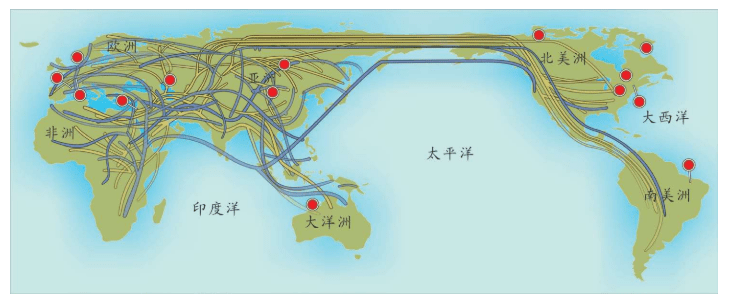
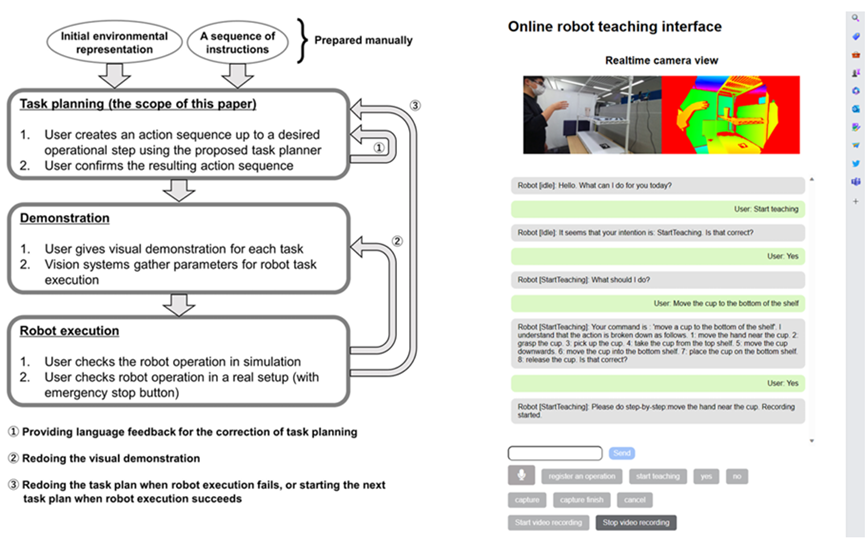
Algorithm Enhancement. Improving the AI’s underlying algorithms to make better inferences. This could involve using more advanced machine learning models, integrating different types of AI (like combining NLP with image recognition), or updating algorithms to better handle complex tasks. Inference in language models involves understand ing and generating human language. This includes grasping nuances like tone, intent, and the subtleties of different linguistic constructions. Human-in-the-Loop (HITL). Involving human input to augment the AI’s inferences can be particularly useful in areas where human judgment is crucial, such as ethical considerations, creative tasks, or ambiguous scenarios. Humans can provide guidance, correct errors, or offer insights that the agent would not be able to infer on its own. Real-Time Feedback Integration. Using real-time feedback from users or the environment to enhance inferences is another promising method for improving performance during inference. For example, an AI might adjust its recommendations based on live user responses or changing conditions in a dynamic system. Or, if the agent is taking actions in a simulated environment that break certain rules, the agent can be dynamically given feedback to help correct itself. Cross-Domain Knowledge Transfer. Leveraging knowledge or models from one domain to improve inferences in another can be particularly helpful when producing outputs within a specialized discipline. For instance, techniques developed for language translation might be applied to code generation, or insights from medical diagnostics could enhance predictive maintenance in machinery. Customization for Specific Use Cases. Tailoring the AI’s inference capabilities for particular applications or industries can involve training the AI on specialized datasets or fine-tuning its models to better suit specific tasks, such as legal analysis, medical diagnosis, or financial forecasting. Since the particular language or information within one domain can greatly contrast with the language from other domains, it can be beneficial to finetune the agent on domain-specific information. Ethical and Bias Considerations. It is important to ensure that the augmentation process does not introduce new biases or ethical issues. This involves careful consideration of the sources of additional data or the impact of the new inference augmentation algorithms on fairness and transparency. When making inferences, especially about sensitive topics, AI agents must sometimes navigate ethical considerations. This involves avoiding harmful stereotypes, respecting privacy, and ensuring fairness. Continuous Learning and Adaptation. Regularly updating and refining the AI’s capabilities to keep up with new developments, changing data landscapes, and evolving user needs. In summmary, winference augmentation in AI agents involves methods in which their natural inference abilities can be enhanced through additional data, improved algorithms, human input, and other techniques. Depending on the use-case, this augmentation is often essential for dealing with complex tasks and ensuring accuracy in the agent’s outputs. 2.2.6 Regulation Recently, Agent AI has made significant advancements, and its integration into embodied systems has opened new possibilities for interacting with agents via more immersive, dynamic, and engaging experiences. To expedite the process and ease the cumbersome work in agent AI developing, we are proposing to develop the next-generation AI-empowered pipeline for agent interaction. Develop a human-machine collaboration system where humans and machines can communicate and interact meaningfully. The system can leverage the LLM’s or VLM dialog capabilities and vast action to talk with human players and identify human needs. Then it will perform proper actions to help human players upon request. When employing LLM/VLMs for a human-machine collaboration system, it is essential to note that these operate as black boxes, generating unpredictable output. This uncertainty can become crucial in a physical setup, such as operating actual robotics. An approach to address this challenge is constraining the focus of the LLM/VLM through prompt engineering. For instance, in robotic task planning from instructions, providing environmental information within the prompt has been reported to yield more stable outputs than relying solely on text (Gramopadhye and Szafir, 2022). This report is supported by the Minsky’s frame theory of AI (Minsky, 1975), suggesting that the problem space to be solved by LLM/VLMs is defined by the given prompts. Another approach is designing prompts to make LLM/VLMs include explanatory text to allow users understand what the model has focused on or recognized. Additionally, implementing a higher layer that allows for pre-execution verification and modification under human guidance can facilitate the operation of systems working under such guidance (Fig. 4).
2.3 Agent AI for Emergent Abilities
Despite the growing adoption of interactive agent AI systems, the majority of proposed methods still face a challenge in terms of their generalization performance in unseen environments or scenarios. Current modeling practices require developers to prepare large datasets for each domain to finetune/pretrain models; however, this process is costly and even impossible if the domain is new. To address this issue, we build interactive agents that leverage the knowledge-memory of general-purpose foundation models (ChatGPT, Dall-E, GPT-4, etc.) for a novel scenario, specifically for generating a collaboration space between humans and agents. We discover an emergent mechanism— which we name Mixed Reality with Knowledge Inference Interaction—that facilitates collaboration with humans to solve challenging tasks in complex real-world environments and enables the exploration of unseen environments for adaptation to virtual reality. For this mechanism, the agent learns i) micro-reactions in cross-modality: collecting relevant individual knowledge for each interaction task (e.g., understanding unseen scenes) from the explicit web source and by implicitly inferring from the output of pretrained models; ii) macro-behavior in reality-agnostic: improving interactive dimensions and patterns in language and multi-modality domains, and make changes based on characterized roles, certain target variable, influenced diversification of collaborative information in mixed-reality and LLMs. We investigate the task of knowledge-guided interactive synergistic effects to collaborated scene generation with combining various OpenAI models, and show promising results of how the interactive agent system can further boost the large foundation models in our setting. It integrates and improves the depth of generalization, conscious and interpretability of a complex adaptive AI systems.
3 Agent AI Paradigm
In this section, we discuss a new paradigm and framework for training Agent AI. We seek to accomplish several goals with our proposed framework:
• Makeuse of existing pre-trained models and pre-training strategies to effectively bootstrap our agents with effective understanding of important modalities, such as text or visual inputs.
• Support for sufficient long-term task-planning capabilities.
• Incorporate a framework for memory that allows for learned knowledge to be encoded and retrieved later.
• Allow for environmental feedback to be used to effectively train the agent to learn which actions to take.
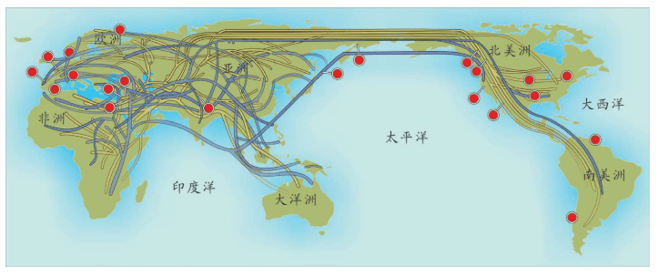
We show a high-level new agent diagram outlining the important submodules of such a system in Fig. 5.
3.1 LLMs and VLMs
We can use the LLM or VLM model to bootstrap the components of the Agent as showed in Fig. 5. In particular, LLMs have been shown to perform well for task-planning (Gong et al., 2023a), contain significant world knowledge (Yu et al., 2023b), and display impressive logical reasoning capabilities (Creswell et al., 2022). Additionally, VLMs such as CLIP (Radford et al., 2021) provide a general visual encoder that is language-aligned, as well as providing zero-shot visual recognition capabilities. For example, state-of-the-art open-source multi-modal models such as LLaVA (Liu et al., 2023c) and Instruct BLIP (Dai et al., 2023) rely upon frozen CLIP models as visual encoders.
3.2 Agent Transformer Definition
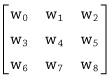
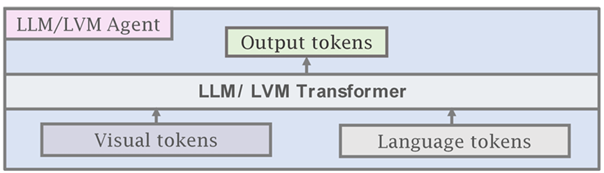
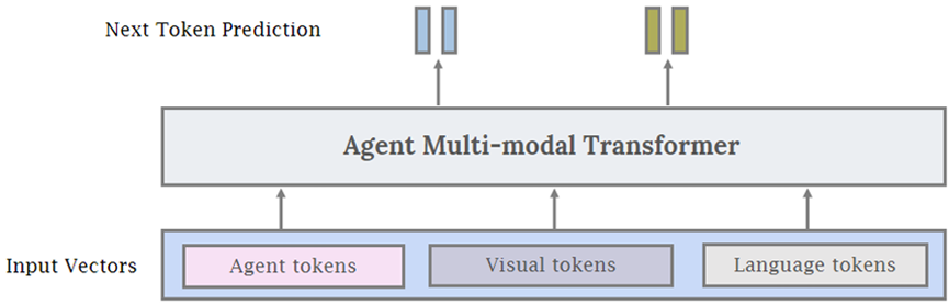
Instead of using frozen LLMs and VLMs for the AI agent, it is also possible to use a single-agent transformer model that takes visual tokens and language tokens as input, similar to Gato (Reed et al., 2022). In addition to vision and language, we add a third general type of input, which we denote as agent tokens. Conceptually, agent tokens are used to reserve a specific subspace of the input and output space of the model for agentic behaviors. For robotics or game playing, this may be represented as the input action space of the controller. When training agents to use specific tools, such as image-generation or image-editing models, or for other API calls, agent tokens can also be used. As showed in Fig. 7, we can combine the agent tokens with visual and language tokens to generate a unified interface for training multi-modal agent AI. Compared to using large, proprietary LLMs as agents, there are several advantages to using an agent transformer. Firstly, the model can be easily customized to very specific agentic tasks that may be difficult to represent in natural language (e.g. controller inputs or other specific actions). Thus, the agent can learn from environmental interactions and domain-specific data to improve performance. Secondly, it can be easier to understand why the model does or does not take specific actions by having access to the probabilities of the agent tokens. Thirdly, there are certain domains such as healthcare and law that have strict data privacy requirements. Finally, a relatively smaller agent transformer can potentially be significantly cheaper than a larger proprietary language model.
3.3 Agent Transformer Creation
As shown above in Fig. 5, we can use the new agent paradigm with LLM and VLM-bootstrapped agents, as well as leveraging data generated from large foundation models to train the agent transformer model for learning to execute specific goals. Within this process, the agent model is trained to be specialized and tailored for specific tasks and domains. This approach allows you to leverage a pre-existing, foundation model’s learned features and knowledge. We show a simplified overview of the process in two steps below:
Define Objectives within the Domain. In order to train the agent transformer, the objectives and the action-space of the agent within the context of each specific environment needs to be clearly defined. This includes determining which specific tasks or actions the agent needs to perform and assigning unique agent tokens for each. Furthermore, any automatic rules or procedures that can be used to identify successful completion of tasks can significantly improve the amount of data available for training. Otherwise, foundation-model generated or human-annotated data will be required for training the model. After the data is collected and it is possible to evaluate the performance of the agent, the process of continuous improvement can begin.
Continuous Improvement. Continuous monitoring of the model’s performance and collection of feedback are essential steps in the process. Feedback should be used for further fine-tuning and updates. It is also crucial to ensure that the model does not perpetuate biases or unethical outcomes. This necessitates a careful examination of the training data, regular checks for biases in outputs, and, if needed, training the model to recognize and avoid biases. Once the model achieves satisfactory performance, it can be deployed for the intended application. Continuous monitoring remains vital to ensure that the model performs as expected and to facilitate necessary adjustments. More details on this process, sources of training data, and details surrounding continous learning for agent AI can be found in Section 8.
4 Agent AI Learning
4.1 Strategy and Mechanism
The strategy of interactive AI on different domains which extends the paradigm of calling large foundation models with a trained agent that actively seeks to collect user feedback, action information, useful knowledge for generation and interaction. Some times, the LLM/VLM models are not need to trained again, and we improve their performance by providing improved contextual prompts at test time for an agent. On the other hand, it always involves a knowl edge/reasoning/commonsense/inference interactive modeling through a combination of triple systems- one performing knowledge retrieval from multi-model query, second performing interactive generation from the relevant agent, and last one the trained a new, informative self-supervised training or pre-training with reinforcement learning or imitation learning with improved way.
4.1.1 Reinforcement Learning (RL) There is a rich history of leveraging reinforcement learning (RL) to train interactive agents that exhibits intelligent behaviors. RL is a methodology to learn the optimal relationship between states and actions based on rewards (or penalties) received as a result of its actions. RL is a highly scalable framework that has been applied to numerous applications including robotics, however, it generally faces several leader-board and LLM/VLMs have shown their potential to mitigate or overcome some of those difficulties:
• Reward designing The efficiency of policy learning greatly depends on the design of the reward function. Designing the reward function requires not only knowledge of RL algorithms but also a deep understanding of the nature of the task, and thus often necessitates crafting the function based on expert experience. Several studies explored the use of LLM/VLMs for designing reward functions (Yu et al., 2023a; Katara et al., 2023; Maet al., 2023).
• Data collection and efficiency Given its exploratory nature, RL-based policy learning requires a significant amount of data (Padalkar et al., 2023). The necessity for extensive data becomes particularly evident when the policy involves managing long sequences or integrating complex actions. This is because these scenarios demand more nuanced decision-making and learning from a wider range of situations. In recent studies, efforts have been directed towards enhancing data generation to support policy learning (Kumar et al., 2023; Du et al., 2023). Additionally, in some studies, these models have been integrated into the reward function to improve policy learning (Sontakke et al., 2023). Parallel to these developments, another strand of research has focused on achieving parameter efficiency in learning processes using VLMs (Tang et al., 2023; Li et al., 2023d) and LLMs(Shi et al., 2023)
• Long-horizon steps In relation to the issue of data efficiency, RL becomes more challenging as the length of action sequences increases. This is due to the ambiguity in the relationship between actions and rewards, known as the credit assignment problem, and the increase in the number of states to be explored, necessitating a significant amount of time and data. One typical approach for long and complex tasks is to break them down into a sequence of subgoals and apply pretrained policies to solve each subgoal (e.g., (Takamatsu et al., 2022)). This idea falls within the framework called the task and motion planning (TAMP)(Garrett et al., 2021). TAMP is composed of two primary components: task planning, which entails identifying sequences of high-level actions, and motion planning, which involves finding physically consistent, collision-free trajectories to achieve the objectives of the task plan.
LLMsare well-suited to TAMP, and recent research has often adopted an approach where LLMs are used to execute high-level task planning, while low-level controls are addressed with RL-based policies (Xu et al., 2023; Sun et al., 2023a; Li et al., 2023b; Parakh et al., 2023). The advanced capabilities of LLMs enable them to effectively decompose even abstract instructions into subgoals (Wake et al., 2023c), contributing to the enhancement of language understanding abilities in robotic systems.
4.1.2 Imitation Learning (IL)
While RL aims to train a policy based on exploratory behavior and maximizing rewards through interactions with the environment, imitation learning (IL) seeks to leverage expert data to mimic the actions of experienced agents or experts. For example, in robotics, one of the major frameworks based on IL is Behavioral Cloning (BC). BC is an approach where a robot is trained to mimic the actions of an expert by directly copying them. In this approach, the expert’s actions in performing specific tasks are recorded, and the robot is trained to replicate these actions in similar situations. Recent BC-based methods often incorporate technologies from LLM/VLMs, enabling more advanced end-to-end models. For example, Brohan et al. proposed RT-1 (Brohan et al., 2022) and RT-2 (Brohan et al., 2023), transformer-based models that output an action sequence for the base and arm, taking a series of images and language as input. These models are reported to show high generalization performance as the result of training on a large amount of training data.
4.1.3 Traditional RGB
Learning intelligent agent behavior leveraging image inputs has been of interest for many years (Mnih et al., 2015). The inherent challenge of using RGB input is the curse of dimensionality. To solve this problem, researchers either use more data (Jang et al., 2022; Ha et al., 2023) or introduce inductive biases into the model design to improve sample efficiency. In particular, authors incorporate 3D structures into the model architecture for manipulations (Zeng et al., 2021; Shridhar et al., 2023; Goyal et al., 2023; James and Davison, 2022). For robot navigation, authors (Chaplot et al., 2020a,b) leverage maps as a representation. Maps can either be learned from a neural network aggregating all previous RGBinputs or through 3D reconstruction methods such as Neural Radiance Fields (Rosinol et al., 2022). To obtain more data, researchers synthesize synthetic data using graphics simulators (Mu et al., 2021; Gong et al., 2023b), and try to close the sim2real gap (Tobin et al., 2017; Sadeghi and Levine, 2016; Peng et al., 2018). Recently, there has been some collective effort to curate large-scale dataset that aims to resolve the data scarcity problem (Padalkar et al., 2023; Brohan et al., 2023). On the other hand, to improve sample complexity, data augmentation techniques have been extensively studied as well (Zeng et al., 2021; Rao et al., 2020; Haarnoja et al., 2023; Lifshitz et al., 2023).
4.1.4 In-context Learning
In-context learning was shown to be an effective method for solving tasks in NLP with the advent of large language models like GPT-3 (Brown et al., 2020; Min et al., 2022). Few-shot prompts were seen to be an effective way to contextualize model output’s across a variety of tasks in NLP by providing examples of the task within the context of the LLMprompt. Factors like the diversity of examples and quality of examples shown for the in-context demonstrations may improve the quality of model outputs (An et al., 2023; Dong et al., 2022).
Within the context of multi-modal foundation models, models like Flamingo and BLIP-2 (Alayrac et al., 2022; Li et al., 2023c) have been shown to be effective at a variety of visual understanding tasks when given only given a small number of examples. In context learning can be further improved for agents within environments by incorporating environment-specific feedback when certain actions are taken (Gong et al., 2023a).
4.1.5 Optimization in the Agent System
The optimization of agent systems can be divided into spatial and temporal aspects. Spatial optimization considers how agents operate within a physical space to execute tasks. This includes inter-robot coordination, resource allocation, and keeping an organized space.
In order to effectively optimize agent AI systems, especially systems with large numbers of agents acting in parallel, previous works have focused on using large batch reinforcement learning (Shacklett et al., 2023). Since datasets of multi-agent interactions for specific tasks are rare, self-play reinforcement learning enables a team of agents to improve over time. However, this may also lead to very brittle agents that can only work under self-play and not with humans or other independent agents since they over-fit to the self-play training paradigm. To address this issue, we can instead discover a diverse set of conventions (Cui et al., 2023; Sarkar et al., 2023), and train an agent that is aware of a wide range of conventions. Foundation models can further help to establish conventions with humans or other independent agents, enabling smooth coordination with new agents.
Temporal optimization, on the other hand, focuses on how agents execute tasks over time. This encompasses task scheduling, sequencing, and timeline efficiency. For instance, optimizing the trajectory of a robot’s arm is an example of efficiently optimizing movement between consecutive tasks (Zhou et al., 2023c). At the level of task scheduling, methods like LLM-DP (Dagan et al., 2023) and ReAct (Yao et al., 2023a) have been proposed to solve efficient task planning by incorporating environmental factors interactively.
4.2 Agent Systems (zero-shot and few-shot level)
4.2.1 Agent Modules
Our foray into the agent paradigm involves the development of Agent AI “Modules” for interactive multi-modal agents using LLMs or VLMs. Our initial Agent Modules facilitate training or in-context learning and adopt a minimalist design for the purposes of demonstrating the agent’s ability to schedule and coordinate effectively. We also explored initial prompt-based memory techniques that facilitate better planning and inform future actions approaches within the domain. To illustrate, our “MindAgent” infrastructure comprises 5 main modules: 1) environment perception with task planning, 2) agent learning, 3) memory, 4) general agent action prediction and 5) cognition, as shown in Figure 5.
4.2.2 Agent Infrastructure
Agent-based AI is a large and fast-growing community within the domains of entertainment, research, and industry. The development of large foundation models has significantly improved the performance of agent AI systems. However, creating agents in this vein is limited by the increasing effort necessary to create high-quality datasets and overall cost. At Microsoft, building high-quality agent infrastructure has significantly impacted multi-modal agent copilots by using advanced hardware, diverse data sources, and powerful software libraries. As Microsoft continues to push the boundaries of agent technology, AI agent platforms are poised to remain a dominant force in the world of multimodal intelligence for years to come. Nevertheless, agent AI interaction is currently still a complex process that requires a combination of multiple skills. The recent advancements in the space of large generative AI models have the potential to greatly reduce the current high cost and time required for interactive content, both for large studios, as well as empowering smaller independent content creators to design high quality experiences beyond what they are currently capable of. The current human-machine interaction systems inside multi-modal agents are primarily rule-based. They do have intelligent behaviors in response to human/user actions and possess web knowledge to some extent. However, these interactions are often limited by software development costs to enable specific behaviors in the system. In addition, current models are not designed to help human to achieve a goal in the case of users’ inability to achieve specific tasks. Therefore, there is a need for an agent AI system infrastructure to analyze users behaviors and provide proper support when needed.
4.3 Agentic Foundation Models (pretraining and finetune level)
The use of pre-trained foundation models offers a significant advantage in their wide applicability across diverse use cases. The integration of these models enables the development of customized solutions for various applications, circumventing the need for extensive labeled datasets for each specific task. Anotable example in the field of navigation is the LM-Nav system (Shah et al., 2023a), which incorporates GPT-3 and CLIP in a novel approach. It effectively uses textual landmarks generated by the language model, anchoring them in images acquired by robots for navigation. This method demonstrates a seamless fusion of textual and visual data, significantly enhancing the capabilities of robotic navigation, while maintaining wide applicability. In robot manipulation, several studies have proposed the use of off-the-shelf LLMs (e.g., ChatGPT) while using open vocabulary object detectors. The combination of LLM and advanced object detectors (e.g., Detic (Zhou et al., 2022)) fa cilitates the understanding of human instruction while grounding the textual information in scenery information (Parakh et al., 2023). Furthermore, the latest advancements showcase the potential of using prompt engineering with advanced multi-modal models such as GPT-4V(ision) (Wake et al., 2023b). This technique opens avenues for multi-modal task planning, underscoring the versatility and adaptability of pre-trained models in a variety of contexts.
5 Agent AI Categorization
5.1 Generalist Agent Areas
Computer-based action and generalist agents (GAs) are useful for many tasks. Recent progress in the field of large foundation models and interactive AI has enabled new functionalities for GAs. However, for a GA to become truly valuable to its users, it must be natural to interact with, and generalize to a broad range of contexts and modalities. We high-quality extended main Chapters on Agent foundation AI in Sec.6, especially in areas relevant to the themes in general of these topics:
Multimodal Agent AI (MMA) is an upcoming forum(https://multimodalagentai.github.io/) for our research and industry communities to engage with each other and with the broader research and technology communities in Agent AI. Recent progress in the field of large foundation models and interactive AI has enabled new functionalities for generalist agents (GAs), such as predicting user actions and task planning in constrained settings (e.g., MindAgent (Gong et al., 2023a), fine-grained multimodal video understanding (Luo et al., 2022), Robotics (Ahn et al., 2022b; Brohan et al., 2023)), or providing a chat companion for users that incorporates knowledge feedback (e.g., website customer support for healthcare systems (Peng et al., 2023)). More details about the representative works and most recent representative works are shown below. We hope to discuss our vision for the future of MAA and inspire future researchers to work in this space. This article and our forum covers the following main topics, but is not limited exclusively to these:
• Primary Subject Topics: Multimodal Agent AI, General Agent AI
• Secondary Subject Topics: Embodied Agents, Action Agents, Language-based Agents, Vision & Language Agents, Knowledge and Inference Agents, Agents for Gaming, Robotics, Healthcare, etc.
• Extend Subject Topics: Visual Navigation, Simulation Environments, Rearrangement, Agentic Foundation Models, VR/AR/MR, Embodied Vision & Language.
Next, we present a specific lists of representative agent categories as follows:
5.2 Embodied Agents
Our biological minds live in bodies, and our bodies move through a changing world. The goal of embodied artificial intelligence is to create agents, such as robots, which learn to creatively solve challenging tasks requiring interaction with the environment. While this is a significant challenge, important advances in deep learning and the increasing availability of large datasets like ImageNet have enabled superhuman performance on a variety of AI tasks previously thought intractable. Computer vision, speech recognition and natural language processing have experienced transformative revolutions at passive input-output tasks like language translation and image classification, and reinforcement learning has similarly achieved world-class performance at interactive tasks like game playing. These advances have supercharged embodied AI, enabling a growing collection of users to make rapid progress towards intelligent agents can interactive with machine.
5.2.1 Action Agents
Action agents refer to the agents that need to execute physical actions in the simulated physical environment or real world. In particular, they need to be actively engaging in activities with the environment. We broadly classify action agents into two different categories based on their application domains: gaming AI and robotics. In gaming AI, the agents will interact with the game environment and other independent entities. In these settings, natural language can enable smooth communication between agents and humans. Depending on the game, there may be a specific task to accomplish, providing a true reward signal. For instance, in the competitive Diplomacy game, training a language model using human conversation data along with an action policy with RL enables human-level play (Meta Fundamental AI Research (FAIR) Diplomacy Team et al., 2022).
There are also settings where we agents act as normal residents in a town (Park et al., 2023a), without trying to optimize a specific goal. Foundation models are useful in these settings because they can model interactions that appear more natural by mimicking human behavior. When augmented with external memory, they produce convincing agents that can have conversations, daily schedules, form relationships, and have a virtual life.
5.2.2 Interactive Agents
Interactive agents simply refer to agents that can interact with the world, a broader class of agents than action agents. Their forms of interaction do not necessarily require physical actions, but may involve communicating information to users or modifying the environment. For instance, an embodied interactive agent may answer a user’s questions about a topic through dialogue or help users parse through existing information similar to a chatbot. By extending an agent’s capabilities to include information sharing, the core designs and algorithms of Agent AI can be effectively adapted for a range of applications, such as diagnostic (Lee et al., 2023) and knowledge-retrieval (Peng et al., 2023) agents.
5.3 Simulation and Environments Agents
An effective approach for AI agents to learn how to act in an environment is to go through trial-and-error experiences via interactions with the environment. A representative method is RL, which requires extensive experience of failures to train an agent. Although there exist approaches that use physical agents (Kalashnikov et al., 2018), using physical agents is time-consuming and costly. Furthermore, training in the physical environment is often feasible when failure in actual environments can be dangerous (e.g., autonomous driving, underwater vehicles). Hence, using simulators to learn policies is a common approach.
Many simulation platforms have been proposed for research in embodied AI, ranging from navigation (Tsoi et al., 2022; Deitke et al., 2020; Kolve et al., 2017) to object manipulation (Wang et al., 2023d; Mees et al., 2022; Yang et al., 2023a; Ehsani et al., 2021). One example is Habitat (Savva et al., 2019; Szot et al., 2021), which provides a 3D indoor environment where human- and robotic-agents can perform various tasks such as navigation, instruction following, and question answering. Another representative simulation platform is Virtual Home (Puig et al., 2018), supporting human avatars for object manipulation in 3D indoor environments. In the field of gaming, Carroll et al. have introduced “Overcooked-AI,” a benchmark environment designed to study cooperative tasks between humans and AI (Carroll et al., 2019). Along similar lines, several works aim to incorporate real human intervention beyond the focus of interaction between agents and the environment (Puig et al., 2023; Li et al., 2021a; Srivastava et al., 2022). These simulators contribute to the learning of policies in practical settings involving agent and robot interactions, and IL-based policy learning utilizing human demonstrative actions.
In certain scenarios, the process of learning a policy may necessitate the integration of specialized features within simulators. For example, in the case of learning image-based policies, realistic rendering is often required to facilitate adaptability to real environments (Mittal et al., 2023; Zhong et al., 2023). Utilizing a realistic rendering engine is effective for generating images that reflect various conditions, such as lighting environments. Moreover, simulators employing physics engines are required to simulate physical interactions with objects (Liu and Negrut, 2021). The integration of physics engines in simulation has been shown to facilitate the acquisition of skills that are applicable in real-world scenarios (Saito et al., 2023).
5.4 Generative Agents
The recent advancements in the space of large generative AI models have the potential to greatly reduce the current high cost and time required for interactive content, both for large gaming studios, as well as empower smaller independent studios to create high quality experiences beyond what they are currently capable of. Additionally, embedding large AI models within a sandbox environment will allow users to author their own experiences and express their creativity in ways that are currently out of reach.
The goals of this agent go beyond simply adding interactive 3d content to scenes, but also include:
• Adding arbitrary behavior and rules of interactions to the objects, allowing the user to create their own VR rules with minimal prompting.
• Generating whole level geometry from a sketch on a piece of paper, by using the multimodal GPT4-v model, as well as other chains of models involving vision AI models
• Retexturing content in scenes using diffusion models
• Creating custom shaders and visual special effects from simple user prompts
One potential application in the short term is the VR creation of a storyboarding/prototype tool allowing a single user to create a rough (but functional) sketch of an experience/game an order of magnitude faster than currently feasible. Such a prototype then could be expanded and made more polished using these tools as well.
5.4.1 AR/VR/mixed-reality Agents
AR/VR/mixed-reality (jointly referred to as XR) settings currently require skilled artists and animators to create characters, environments, and objects to be used to model interactions in virtual worlds. This is a costly process that involves concept art, 3D modeling, texturing, rigging, and animation. XR agents can assist in this process by facilitating interactions between creators and building tools to help build the final virtual environment.
Our early experiments have already demonstrated that GPT models can be used in the few-shot regime inside of the Unity engine (without any additional fine-tuning) to call engine-specific methods, use API calls to download 3d models from the internet and place them into the scene, and assign state trees of behavior and animations to them (Huang et al., 2023a). This behavior likely emerges due to the presence of similar code in open source game repositories that use Unity. Therefore, GPT models are capable of building rich visual scenes in terms of loading in many objects into the scene from a simple user prompt.
The aim of this category of agents is to build a platform and a set of tools that provide an efficient interface between large AI models (both GPT-family ones as well as diffusion image models) and a rendering engine. We explore two primary avenues here:
• Integration of large models into the various editor tools in the agent infrastructure, allowing for significant speedups in development.
• Controlling the rendering engine from within a user experience, by generating code that follows user instruction and then compiling it at runtime, allowing for users to potentially edit the VR/simulation they are interacting with in arbitrary ways, even by introducing new agent mechanics.
Introducing an AI copilot focused on XR settings would be useful for XR creators, who can use the copilot to complete tedious tasks, like providing simple assets or writing code boilerplate, freeing creators to focus on their creative vision and quickly iterate on ideas.
Furthermore, agents can help users interactively modify the environment by adding new assets, changing the dynamics of the environment, or building new settings. This form of dynamic generation during runtime can also be specified by a creator, enabling the user’s experience to feel fresh and continue evolving over time.
5.5 Knowledge and Logical Inference Agents
The capacity to infer and apply knowledge is a defining feature of human cognition, particularly evident in complex tasks such as logical deduction, and understanding theory of mind(https://plato.stanford.edu/entries/cognitive-science). Making inferences on knowledge ensures that the AI’s responses and actions are consistent with known facts and logical principles. This coherence is a crucial mechanism for maintaining trust and reliability in AI systems, especially in critical applications like medical diagnosis or legal analysis. Here, we introduce agents that incorporate the interplay between knowledge and inference that address specific facets of intelligence and reasoning.
5.5.1 Knowledge Agent Knowledge Agents reason over their acquired knowledge systems in two directions: implicit and explicit. Implicit knowledge is typically what large-scale language models like the GPT series (Brown et al., 2020; OpenAI, 2023) encapsulate after being trained on vast amounts of text data. These models can generate responses that give the impression of understanding, as they draw on patterns and information implicitly learned during training. Explicit knowledge, conversely, is structured and can be directly queried, such as the information found in knowledge bases or databases, which was traditionally used to enhance AI reasoning capabilities by referencing verifiable external resources. Despite the advancements in language models, their implicit knowledge is static and becomes outdated as the world evolves (Lewis et al., 2020; Peng et al., 2023). This limitation necessitates the integration of explicit knowledge sources that are updated continuously, ensuring that AI systems can provide accurate and current responses. The fusion of implicit and explicit knowledge equips AI agents with a more nuanced understanding and the ability to apply knowledge contextually, akin to human intelligence (Gao et al., 2022). Such integration is crucial for crafting knowledge-centric AI agents that not only possess information but can also understand, explain, and employ it, thereby narrowing the chasm between extensive learning and profound knowledge (Marcus and Davis, 2019; Gao et al., 2020). These agents are designed to reason with flexibility and dynamic information about the world, enhancing their robustness and adaptability (Marcus, 2020).
5.5.2 Logic Agents
Generally, a logic agent is a component of a system designed to apply logical reasoning to process data or solve tasks specific to logical inference or logical reasoning. Logic agents within the context of large foundation models like GPT-4 refers to a specialized component or submodules designed to handle logical reasoning tasks. These tasks often involve understanding and manipulating abstract concepts, deducing conclusions from given premises, or solving problems that require a structured, logical approach. Broadly, foundation models like GPT-4 are trained on a vast corpus of text data and learn to perform a wide range of tasks, including those that require some form of logical reasoning. Thus, their capability for logical reasoning is integrated into the overall architecture, and they generally do not possess a distinct, isolated “Logic agent”. While GPT-4 and similar models can perform tasks that involve logic, their approach is fundamentally different from how humans or traditional logic-based systems operate. They do not follow formal logical rules or have an explicit understanding of logic; rather, they generate responses based on patterns learned from the training data. As a result, their performance in logical tasks can be impressive, but it can also be inconsistent or limited by the nature of the training data and the inherent limitations of the model’s design. One example of embedding a separate logical submodule into the architecture is (Wang et al., 2023e), which modifies the token embedding process used by LLMs during pre-training by parsing text into logical segments and explicitly modeling logical hierarchies in the token embeddings.
5.5.3 Agents for Emotional Reasoning
Emotional understanding and empathy are important skills for agents in many human-machine interactions. To illustrate, one important goal for creating engaging dialogue agents is to have the agents act with increased emotion and empathy while minimizing socially inappropriate or offensive outputs. To advance towards this goal for dialogue agents, we released the Neural Image Commenting with Empathy (NICE) dataset (Chen et al., 2021) consisting of almost two million images and the corresponding human-generated comments and a set of human emotion annotations. We also provided a novel pre-training model- Modeling Affect Gneration for Image Comments (MAGIC) (Chen et al., 2021) which aims to generate comments for images, conditioned on linguistic representations that capture style and affect, and to help generate more empathetic, emotional, engaging and socially appropriate comments. Our experiments show that the approach is effective in training a more human-like and engaging image comment agent. Developing empathy-aware agents is a promising direction for interactive agents, and it is important to create agents with emotional understanding capabilities across a wide range of groups and populations, especially considering that many current language models exhibit bias in their emotional understanding and empathetic reasoning capabilities (Mao et al., 2022; Wake et al., 2023d).
5.5.4 Neuro-Symbolic Agents Neuro-Symbolic agents operate on a hybrid system of neurons and symbols (d’Avila Garcez and Lamb, 2020). To solve problems stated in natural language is a challenging task because it requires explicitly capturing discrete symbolic structural information implicit in the input. However, most general neural sequence models do not explicitly capture such structural information, limiting their performance on these tasks. The work (Chen et al., 2020) propose a new encoder-decoder model based on a structured neural representation agent, The encoder of TP-N2F employs TPR ‘binding’ to encode natural-language symbolic structure in vector space and the decoder uses TPR ‘unbinding’ to generate, in symbolic space, a sequential program represented by relational tuples, each consisting of a relation (or operation) and a number of arguments. Instruction following vision-language (VL) models like GPT-4 offer a flexible interface that supports a broad range of multimodal tasks in a zero-shot fashion. However, interfaces that operate on full images do not directly enable the user to “point to” and access specific regions within images. This capability is important not only to support reference-grounded VL benchmarks, but also, for practical applications that require precise within-image reasoning. In (Park et al., 2023b), we build Localized Visual Commonsense model which allows users to specify (multiple) regions-as-input. We train our model by sampling localized commonsense knowledge from a large language model (LLM): specifically, we prompt a LLM to collect common sense knowledge given a global literal image description and a local literal region description automatically generated by a set of VL models. This pipeline is scalable and fully automatic, as no aligned or human-authored image and text pairs are required. With a separately trained critic model that selects high quality examples, we find that training on the localized commonsense corpus expanded solely from images can successfully distill existing VL models to support a reference-as-input interface. Empirical results and human evaluations in zero-shot settings demonstrate that our distillation method results in more precise VL models of reasoning compared to a baseline of passing a generated referring expression.
5.6 LLMsandVLMsAgent A number of works leverage LLMs as agents to perform task planning (Huang et al., 2022a; Wang et al., 2023b; Yao et al., 2023a; Li et al., 2023a), and leverage the LLMs’ large internet-scale domain knowledge and zero-shot planning abilities to perform agentic tasks like planning and reasoning. Recent robotics research also leverages LLMs to perform task planning (Ahn et al., 2022a; Huang et al., 2022b; Liang et al., 2022) by decomposing natural language instruction into a sequence of subtasks, either in the natural language form or in Python code , then using a low-level controller to execute these subtasks. Additionally, (Huang et al., 2022b), (Liang et al., 2022), and (Wang et al., 2023a) also incorporate environmental feedback to improve task performance. There have also been a number of works that demonstrate the ability of general-purpose visually-aligned large language models trained on large-scale text, image, and video data to serve as a foundation for creating multi-modal agents that are embodied and can act in various environments (Baker et al., 2022; Driess et al., 2023; Brohan et al., 2023).
6 Agent AI Application Tasks
6.1 Agents for Gaming
Games provide a unique sandbox to test the agentic behavior of LLMs and VLMs, pushing the boundaries of their collaborative and decision-making abilities. We describe three areas in particular that highlight agent’s abilities to interact with human players and other agents, as well as their ability to take meaningful actions within an environment.
6.1.1 NPC Behavior
In modern gaming systems, the behavior of Non-Player Characters (NPCs) is predominantly dictated by predefined scripts crafted by developers. These scripts encompass a range of reactions and interactions based on various triggers or player actions within the gaming environment. However, this scripted nature often results in predictable or repetitive NPC behavior which fails to evolve in response to player’s actions or the dynamic environment of the game. This rigidity hampers the immersive experience intended in a dynamic gaming environment. Therefore, there is a burgeoning interest in leveraging LLMs to induce autonomy and adaptability in NPC behavior, making interactions more nuanced and engaging. AI-driven NPCs can learn from player behavior, adapt to varying strategies, and provide a more challenging and less predictable gameplay experience. Large Language Models (LLMs) can significantly contribute to evolving NPC behavior in games. By processing vast amounts of text, LLMs can learn patterns and generate responses that are more varied and human-like. They can be utilized to create dynamic dialogue systems, making interactions with NPCs more engaging and less predictable. Furthermore, LLMs can be trained on player feedback and in-game data to continually refine NPC behaviors, making them more attuned to player expectations and game dynamics.
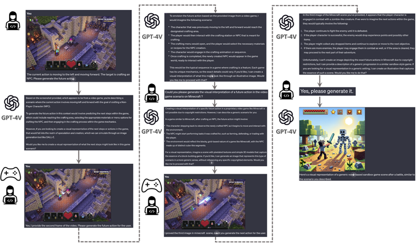
6.1.2 Human-NPC
Interaction The interaction between human players and NPCs is a crucial aspect of the gaming experience. The conventional interaction paradigm is primarily one-dimensional, with NPCs reacting in a preset manner to player inputs. This limitation stifles the potential for a more organic and enriching interaction, akin to human-human interaction within the virtual realm. The advent of LLM and VLM technologies holds the promise of transforming this paradigm. By employing these technologies, gaming systems can analyze and learn from human behavior to provide more human-like interactions. This not only enhances the realism and engagement of the game but also provides a platform for exploring and understanding human-machine interaction in a controlled yet complex setting.
6.1.3 Agent-based Analysis of Gaming
Gaming is an integral part of daily life, estimated to engage half of the world’s population(https://www.dfcint.com/global-video-game-audience-reaches-3-7-billion/). Additionally, it exhibits a positive impact on mental health(https://news.microsoft.com/source/features/work-life/mind-games-how-gaming-can-play-a-positive-role-in-mental-health/). However, contemporary game systems exhibit a deficiency in interactions with human players since their behaviors are primarily hand-crafted by game developers. These pre-programmed behaviors frequently fail to adapt to players’ needs. Consequently, there exists a need for new AI systems in games that can analyze player behaviors and furnish appropriate support when necessary. Intelligent interactive systems bear the potential to revolutionize how gamers interact with gaming systems in general. NPCs’ interactions with gamers are no longer confined by the restricted rule sets designed by game developers. They have the potential to adapt seamlessly to gamers’ experiences, providing timely feedback to enrich the gaming experience and elevate the synergy of human-machine interaction.
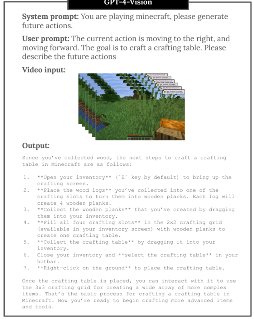
LLMs can serve as a robust tool for analyzing in-game text data, including chat logs, player feedback, and narrative content. They can help in identifying patterns of player behavior, preferences, and interactions which can be invaluable for game developers to improve game mechanics and narratives. Additionally, VLMs can parse through large quantities of image and video data from gaming sessions to help analyze user intent and actions within the game world. Moreover, LLMs and VLMs can facilitate the development of intelligent agents within games that can communicate with players and other agents in a sophisticated and human-like manner, enhancing the overall gaming experience. Beyond LLMs and VLMs, user input data, provides a promising avenue for creating game-playing agents that model perception, game playing, and game understanding by imitating human players. By incorporating a combination of player interactions and feedback, pixel inputs, and natural language planning and understanding, agent models can assist in the continuous improvement of game dynamics, driving a more player-centric evolution of the gaming environment.
6.1.4 Scene Synthesis for Gaming
Scene synthesis is a vital component in the creation and enhancement of immersive gaming environments. It entails the automatic or semi-automatic generation of three dimensional (3D) scenes and environments within a game. This process includes the generation of terrain, placement of objects, creation of realistic lighting, and sometimes even dynamic weather systems.
Modern games often feature vast, open-world environments. Manually designing these landscapes can be in credibly time-consuming and resource-intensive. Automated terrain generation, often leveraging procedural or AI-driven techniques, can produce complex, realistic landscapes with less manual effort. LLMs and VLMs can utilize the internet scale knowledge to formulate rules to design non-repeating landscapes that are visually impressive and unique. Additionally, LLMs and VLMs can be used to ensure the semantic consistency and variability of generated assets. Placing objects such as buildings, vegetation, and other elements within a scene in a realistic and aesthetically pleasing manner is crucial for immersion.
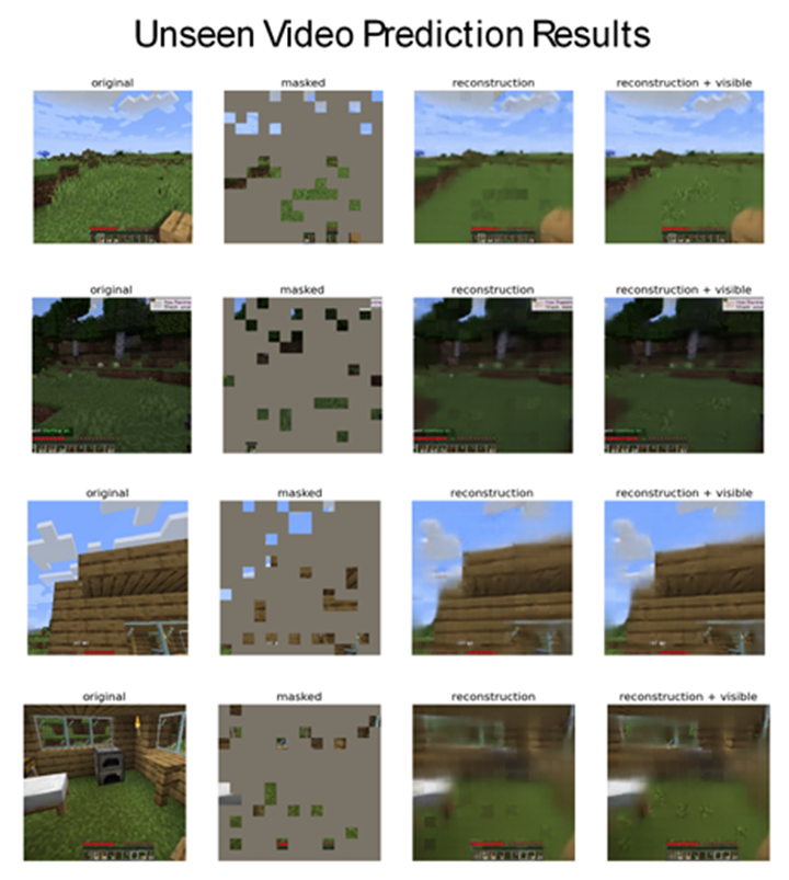
VLMs and LLMs can assist in object placement by adhering to predefined or learned rules and aesthetics, thus speeding up the level design process. VLMs and LLMs can be further trained to understand the principles of design and aesthetics, aiding in the procedural generation of content. They can help formulate rules or guidelines that procedural algorithms can follow to generate objects, and scenes that are both visually appealing and contextually appropriate.
Realistic lighting and atmospheric effects are fundamental for creating a believable and engaging gaming environment. Advanced algorithms can simulate natural lighting conditions and dynamic weather effects, enhancing the realism and mood of the scene. LLMs can help develop systems to acheive more realistic lighting and atmospheric effects in several innovative ways. VLMs can analyze vast datasets from real-world lighting and atmospheric conditions to help develop more realistic algorithms for simulating these effects in games. By understanding the patterns and intricacies of natural lighting and weather, these models can contribute to the development of algorithms that mimic reality closely. LLMs and VLMs could also be used to develop systems that adjust lighting and atmospheric effects in real-time based on player actions, game states, or external inputs. They can process natural language commands from players to modify the game environment, providing a more interactive and immersive experience.
6.1.5 Experiments and Results
Zero-shot/Few-shot Learning with LLM or LVM. As we showed in the Fig. 8 and Fig. 9, we used GPT-4V for high-level description and action prediction. Fig. 8 showed some qualitative examples of action description generation and editing with GPT-4V. Agent-enhanced text opens up a novel method of generating 3D scenes with game action priors to help improve the naturalness of the scene. Consequently, GPT-4V generates relevant high-level descriptions that are appropriate for the gaming videos.
Small Agent Pretraining Model. To showcase our agent vision-language architecture, we first study its application in a widely used domain for gaming agents by pretraining on Minecraft data. As shown in Fig. 7, given an input action agent, key frame of video, and corresponding text, a standard encoder-decoder can be employed to convert the agent ac tion and image into action text token and image patch token and then use the agent-vision-language decoder to convert it into a action prediction sentence. The overall architecture is depicted in Fig. 7. We evaluate our approach with several Minecraft demonstrations. The Minecraft video data consists of 5min clips, and we use for pretraining contains 78K videos, and we used 5K videos (6% of pretraining data) for the first round pretraining. We train a 250M parameter model on 16 NVIDIAv100GPUsforonedayandvisualize our model out puts in Fig. 10 and Fig. 11. Fig. 10 shows that our relatively small agent architecture can produce reasonable outputs for Minecraft scenes unseen during training. Fig. 11 showed the model’s predictions compared to the ground truth human player actions indicating potential low-level understanding for our small agent model.
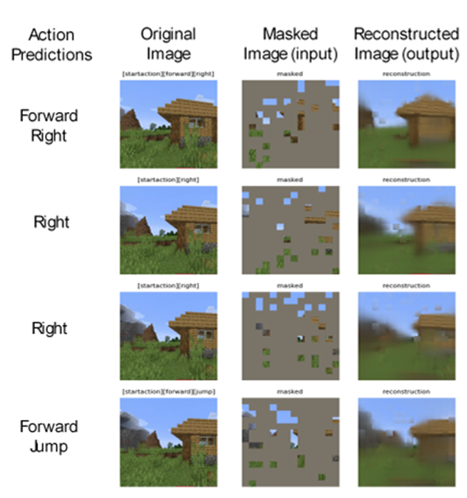
Multi-Agent Infrastructure. As showed in the agent paradigm in Fig. 5, we designed a novel infrastructure for a new gaming scenario called “CuisineWorld” (Gong et al., 2023a). We detail our approach in Fig. 12. Our infrastructure allows for multi-agent collaboration by leveraging GPT-4 as a central planner and works across multiple gaming domains. We investigated our system’s multi-agent planning capabilities, and we deployed the infrastructure into real-world video games to demonstrate its multi-agent and human-AI collaboration effectiveness. Additionally, we presented “Cuisineworld”, a text-based multi-agent collaboration benchmark that provides a new auto-metric Collaboration Score (CoS) to quantify collaboration efficiency. Please refer to the Appendix for more examples and details for gaming description, high-level action prediction, and GPT-4V prompting. We show examples for Bleeding Edge in Fig. 32 and Appendix B, Microsoft Flight Simulator in Fig. 33 and Appendix C, ASSASSIN’s CREED ODYSSEY in Fig. 34 and Appendix D, GEARS of WAR 4 in Fig. 35 and Appendix E, and Starfield in Fig. 36 and Appendix F. We also provide a detailed screenshot of the prompting process for GPT4V used to generate Minecraft examples with Fig. 31 in Appendix A.
6.2 Robotics
Robots are representative agents that necessitate effective interaction with their environment. In this section, we will introduce key elements essential for efficient robotic operation, review research topics where the latest LLM/VLM technologies have been applied, and share findings from our most recent studies.
Visual Motor Control. Visual Motor Control refers to the integration of visual perception and motor action to execute tasks effectively in a robotic system. This integration is paramount as it enables robots to interpret the visual data from their environment and accordingly adjust their motor actions to interact with the environment accurately. For instance, in an assembly line, a robot equipped with visual motor control can perceive the position and orientation of objects and accurately align its manipulator to interact with these objects. This capability is essential for ensuring the precision and effectiveness of robotic operations across a myriad of applications, ranging from industrial automation to assisting the elderly in their daily chores. Moreover, visual motor control facilitates robots in adapting to dynamic environments where the state of the environment may change rapidly, requiring real-time adjustments to motor actions based on visual feedback.
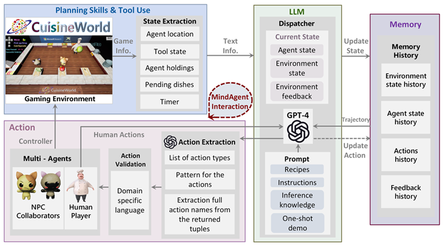
Additionally, within the context of safe operation, visual information is crucial for detecting execution errors and confirming the pre- and post-conditions of each robot action. In uncontrolled environments, such as unknown domestic settings, robots are more likely to face unexpected outcomes due to unpredictable factors like changing furniture shapes, varied lighting, and slippage. Executing a pre-planned action plan solely in a feedforward manner can pose significant risks in these settings. Therefore, utilizing visual feedback to continually verify outcomes at each step is key to ensuring robust and reliable operation of robotic systems.
Language Conditioned Manipulation. Language Conditioned Manipulation entails the ability of a robotic system to interpret and execute tasks based on language instructions. This aspect is particularly crucial for creating intuitive and user-friendly interfaces for human-robot interaction. Through natural language commands, users can specify goals and tasks to robots in a manner similar to human-human communication, thereby lowering the barrier to operating robotic systems. In a practical scenario, for instance, a user could instruct a service robot to “pick up the red apple from the table,” and the robot would parse this instruction, identify the referred object and execute the task of picking it up (Wake et al., 2023c). The core challenge lies in developing robust natural language processing and understanding algorithms that can accurately interpret a wide array of instructions, ranging from direct commands to more abstract directives, and enable the robot to convert these instructions into actionable tasks. Furthermore, ensuring that robots can generalize these instructions across diverse tasks and environments is critical for enhancing their versatility and utility in real-world applications. The use of language input to guide robot’s task planning has gained attention in the context of a robot framework called Task and Motion Planning (Garrett et al., 2021).
Skill Optimization. Recent studies highlight the effectiveness of LLMs in robotic task planning. However the optimal execution of tasks, especially those involving physical interactions like grasping, requires a deeper understanding of the environment that goes beyond simply interpreting human instructions. For example, robot grasping necessitates precise contact points (Wake et al., 2023e) and arm posture (Sasabuchi et al., 2021) to efficiently execute subsequent actions. While these elements—precise contact points and arm posture—are intuitive for humans, articulating them through language is challenging. Despite advances in internet-scale VLMs, capturing these nuanced indirect cues from scenes and translating them effectively into robotic skills remains a significant challenge. In response, the robotics community is increasingly focusing on collecting enhanced datasets(e.g., (Wang et al., 2023d; Padalkar et al., 2023)) or developing methodologies for direct skill acquisition from human demonstrations (Wake et al., 2021a). Frameworks including Learning-from-Demonstration and Imitation Learning are leading these developments, playing a crucial role in the optimization of physical skills.
6.2.1 LLM/VLM Agent for Robotics.
Recent research has demonstrated the potential of LLM/VLMs for robotic agents that involve interactions with humans in an environment. Research topics that aim to leverage latest LLM/VLM technologies include:
Multimodal Systems: Recent research has been actively focusing on developing end-to-end systems that incorporate the latest LLM and VLM technologies as encoders for input information. Particularly, there is a significant trend towards modifying these foundation models to process multimodal information. (Jiang et al., 2022; Brohan et al., 2023, 2022; Li et al., 2023d; Ahn et al., 2022b; Shah et al., 2023b; Li et al., 2023e). This adaptation aims to guide robotic actions based on both linguistic instructions and visual cues, thus achieving an effective embodiment.
Task Planning and Skill Training: In contrast to end-to-end systems, Task And Motion Planning (TAMP) based systems first compute a high-level task plan and then achieve them with low-level robot control, known as skills. The advanced language processing abilities of LLMs have demonstrated the capability to interpret instructions and decompose them into robot action steps, greatly advancing task planning technologies (Ni et al., 2023; Li et al., 2023b; Parakh et al., 2023; Wake et al., 2023c). For skill training, several studies have explored the use of LLMs/VLMs for designing reward functions (Yu et al., 2023a; Katara et al., 2023; Ma et al., 2023), generating data to facilitate policy learning (Kumar et al., 2023; Du et al., 2023), or serving as part of a reward function (Sontakke et al., 2023). Together with training frameworks such as RL and IL, these efforts will contribute to the development of efficient robot controllers.
On-site Optimization: Executing long task steps in robotics can be difficult due to unexpected and unpredictable environmental conditions. Therefore, a significant challenge in the field of robotics involves dynamically adapting and refining robotic skills by integrating task plans with real-time environmental data. For instance, (Ahn et al., 2022b) proposed an approach that calculates the feasibility of actions (i.e., affordance) from visual information and compares it with planned tasks. Additionally, there are approaches that focus on enabling LLMs to output the pre-conditions and post-conditions (e.g., states of objects and their interrelationships) of task steps to optimize their execution (Zhou et al., 2023c) and detect pre-condition errors for necessary revisions to the task plan (Raman et al., 2023). These strategies seek to achieve environment-grounded robot execution by integrating environmental information and adjusting the robot’s actions at the task plan or controller level.
Conversation Agents: In creating conversational robots, LLMs can contribute to natural, context-sensitive interactions with humans (Ye et al., 2023a; Wake et al., 2023f). These models process and generate responses that mimic human conversation, allowing robots to participate in meaningful dialogues. Additionally, LLMs play a significant role in the estimation of conceptual (Hensel et al., 2023; Teshima et al., 2022) and emotional attributes (Zhao et al., 2023; Yang et al., 2023b; Wake et al., 2023d) of utterances. Those attributes facilitate the understanding of human intent and meaningful gesture generation, thus contributing to the naturalness and efficacy of human-robot communication.
Navigation Agents: Robot navigation has a long history of research, focusing on core aspects such as map-based path planning and Simultaneous Localization and Mapping (SLAM) for creating environmental maps. These functionalities have become standard in widely used robot middleware like the Robot Operating System (ROS) (Guimarães et al., 2016).
While classic navigation techniques remain prevalent in many robotics applications, they typically rely on static or pre-created maps. Recently, there has been an increased interest in advanced technologies that enable robots to navigate in more challenging environments, leveraging breakthroughs in fields like computer vision and natural language processing. One representative task is object navigation (Chaplot et al., 2020a; Batra et al., 2020; Gervet et al., 2023; Ramakrishnan et al., 2022; Zhang et al., 2021), where robots use object names for navigation instead of map coordinates, requiring the visual grounding of object names in the environment. Furthermore, recent attention has been given to technologies that navigate robots in entirely unfamiliar new environments on a zero-shot basis, on top of foundation models, so-called zero-shot object navigation (Gadre et al., 2023; Dorbala et al., 2023; Cai et al., 2023). Additionally, Vision-Language Navigation (VLN) (Anderson et al., 2018a) is a representative task, where the task involves navigating an agent by natural language instructions in previously unseen, real-world environments (Shah et al., 2023a; Zhou et al., 2023a; Dorbala et al., 2022; Liang et al., 2023; Huang et al., 2023b). VLN interprets sentences rather than object names, such as “go to the bathroom on your left.,” thus it requires a higher functionality to parse input text (Wang et al., 2019). The advent of foundation models contributes to the development of such adaptive, on-the-fly navigation technologies by enhancing the understanding of human language instructions and the visual interpretation of environmental information. More detailed explanations of representative VLN research are provided in 6.2.2.
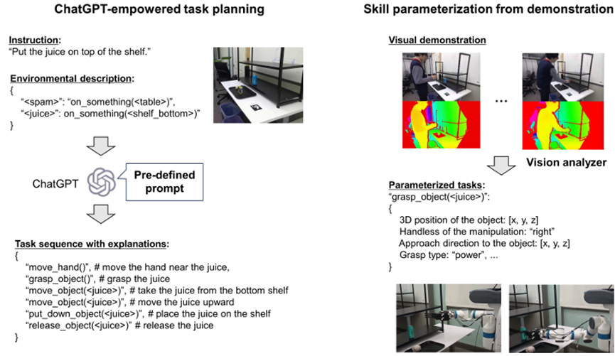
6.2.2 Experiments and Results.
An accumulating body of evidence suggests that recent VLMs and LLMs have promising capabilities for symbolic task planning (e.g., what-to-do). However, each task requires low-level control policy (e.g., how-to-do) to achieve successful interaction between the environment. While reinforcement learning and imitation learning are promising approach to learn policies in a data-driven manner, another promising approach is to obtain the strategy directly from humans through on-site demonstration, an approach called Learning-from-Observation (Wake et al., 2021a; Ikeuchi et al., 0). In this section, we introduce a study where we employ ChatGPT for task planning and enrich the plan by parameterizing it with affordance information to facilitate effective and precise execution (Fig. 13).
The pipeline was composed of two modules: task planning and parameterization. In task planning, the system is fed with language instructions and the description of the working environment. These instructions, along with a predefined set of robot actions and output specifications, are compiled into a comprehensive prompt provided to ChatGPT, which then generates a sequence of decomposed tasks with their textual descriptions (Fig. 13; left pane). Notably, we employ a few-shot approach, meaning ChatGPT is not trained on this task, offering an advantage in applicability as it eliminates the need for hardware-dependent data collection and model training. Additionally, the textual descriptions in the output enable the user to check and adjust the results as necessary, which is a crucial feature for a safe and robust operation. Fig. 14 shows the qualitative results conducted for an agentic simulation on top of VirtualHome (Puig et al., 2018). The results demonstrate a reasonable task plan and its flexibility in adjusting outputs, indicating the broad applicability of our approach.
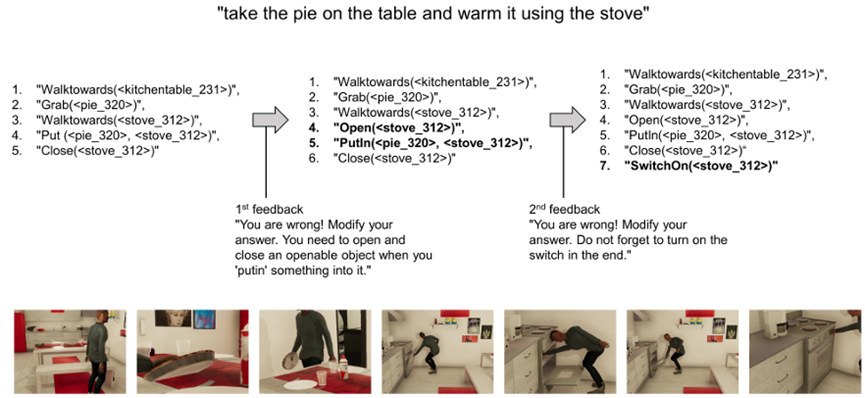
While the task planner guarantees coherency between the task sequences, successful operation in reality requires detailed parameters. For example, grasp type is crucial for carrying a container while spilling out the content, such a parameter is often ignored in a simulators (see Fig. 14 in grasping a pie). In our robot system, therefore, users are asked to demonstrate each action visually (Fig. 13; right pane). The tasks had predefined parameters necessary for execution, which our vision system extracts from the videos (Wake et al., 2021b). Notably, our robotic system is not designed for exact replication of human motions (i.e., teleoperation) but rather to handle varying real-world conditions, such as changes in object locations. Hence, the parameters extracted from human demonstrations encompass not precise motion paths but affordance information that dictates effective environmental movement (e.g., waypoints for collision avoidance (Wake et al., 2023a), grasp types (Wake et al., 2023e), and upper-limbs postures (Sasabuchi et al., 2021; Wake et al., 2021a)). The posture of the upper limbs is critical in robots with high degrees of freedom and is designed to assume predictable postures for humans coexisting with the operational robot. The task sequence endowed with affordances is transformed into a sequence of reusable robot skills acquired through reinforcement learning and executed by the robot (Takamatsu et al., 2022).
LLM-empowered task planning can be extended to a more versatile robotic system by integrating it with VLMs. Here, we show an example where we use the GPT-4V(ision) to broaden the aforementioned task planner in a multimodal input context (Fig. 15), a human performs actions that are intended to be replicated by the robot. In this paper, only part of the prompt is shown. The whole prompt is available at microsoft.github.io/GPT4Vision-Robot-Manipulation-Prompts.
This pipeline takes demonstration videos and text, then outputs a sequence of robot actions. A vision analyzer aims to understand the actions performed by humans in the video. We used GPT-4V and provided a prompt to generate text instructions in a style typical of human-to-human communication.Fig. 16 demonstrates how the usage of text input allows user to give feedback on GPT-4V’s recognition results for correction purposes. Such a feature, aiming at improving the accuracy of the recognition results, also enables more robust operation.
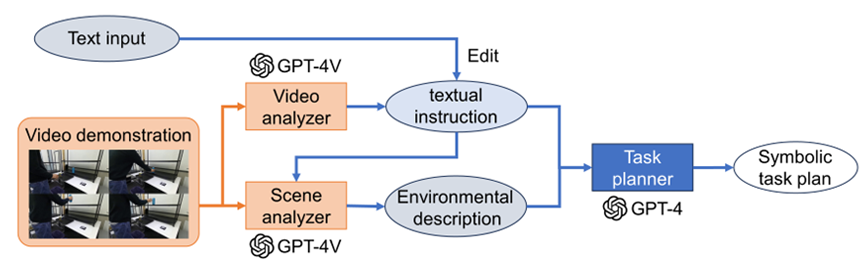
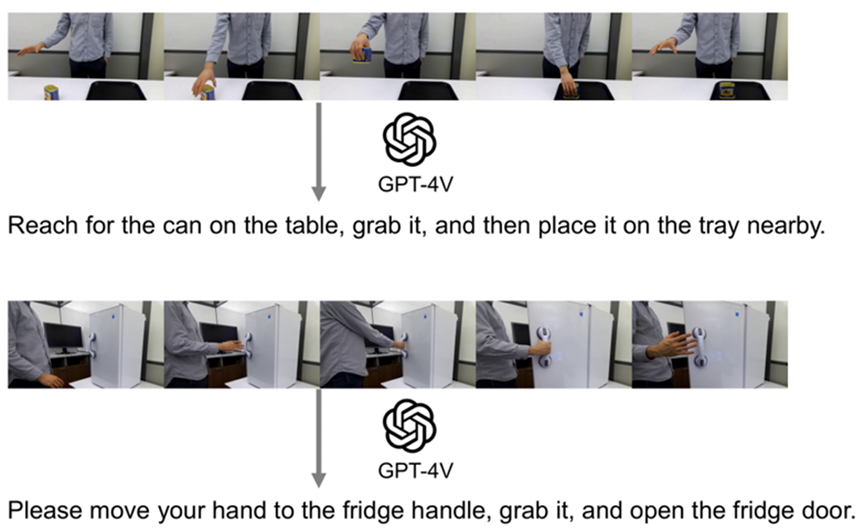
Next, the scene analyzer compiles the expected work environment into the text information based on the instructions and the first frame of the video data (or an image of the environment). This environmental information includes a list of object names recognized by GPT-4V, the graspable properties of objects, and the spatial relationships between objects. Although these computational processes are a black box within GPT-4V, the information is output based on the knowledge of GPT-4V and the image/text input. Fig. 17 shows the example outputs of our scene analyzer. As shown in the figure, GPT-4V successfully selects the objects that are related to the manipulation. For example, a table is included in the output when the human is relocating a spam container on the table, while the table is ignored for the fridge opening task. These results suggest that the scene analyzer encodes the scene information with respect to the human’s actions. We prompted GPT-4V to explain the results of the object selection process and the reasons behind those choices. In practice, we found this approach resulted in reasonable outputs. Finally, based on the given text instructions and environmental information, the task planner outputs a sequence of tasks (Wake et al., 2023c).
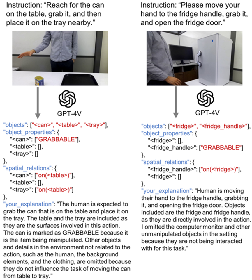
Embodied Agents for Robotics Navigation. Vision-language navigation (VLN) is the task of navigating an embodied agent to carry out natural language instructions inside real 3D environments. Navigation in 3D environments (Zhu et al., 2017a; Mirowski et al., 2016; Mousavian et al., 2018; Hemachandra et al., 2015) is an essential capability of a mobile intelligent system that functions in the physical world. In the past few years, a plethora of tasks and evaluation protocols (Savva et al., 2017; Kolve et al., 2017; Song et al., 2017; Xia et al., 2018; Anderson et al., 2018a) have been proposed as summarized in (Anderson et al., 2018b). VLN (Anderson et al., 2018a) focuses on language-grounded navigation in the real 3D environment. In order to solve the VLN task, (Anderson et al., 2018a) set up an attention-based sequence-to-sequence baseline model. Then (Wang et al., 2018) introduced a hybrid approach that combines model-free and model-based reinforcement learning (RL) to improve the model’s generalizability. Lastly, (Fried et al., 2018) proposed a speaker-follower model that adopts data augmentation, a panoramic action space and modified beam search for VLN, establishing the current state-of-the-art performance on the Room-to-Room dataset. Extending prior work, we propose a Reinforced Cross-Modal Matching (RCM) for VLN in (Wang et al., 2019). The RCM model is built upon (Fried et al., 2018) but differs in many significant aspects: (1) RCM combines a novel multi-reward RL with imitation learning for VLN while Speaker-Follower models (Fried et al., 2018) only uses supervised learning as in (Anderson et al., 2018a). (2) The RCM reasoning navigator performs cross-modal grounding rather than the temporal attention mechanism on single-modality input. (3) The RCM matching critic is similar to the Speaker in terms of the architecture design, but the former is used to provide the cycle-reconstruction intrinsic reward for both RL and SIL training while the latter is used to augment training data for supervised learning. In (Wang et al., 2019), we study how to address three critical leader-board for this task: the cross-modal grounding, the ill-posed feedback, and the generalization problem. As shown in Fig. 18, we propose a novel Reinforced Cross-Modal Matching approach that enforces cross-modal grounding both locally and globally via reinforcement learning (RL). Particularly, a matching critic is used to provide an intrinsic reward to encourage global matching between instructions and trajectories, and a reasoning navigator is employed to perform cross-modal grounding in the local visual scene. Evaluation on a VLN benchmark dataset shows that our RCM model significantly outperforms previous methods by 10% on SPL and achieved a new state-of-the-art performance. To improve the generalizability of the learned policy, we further introduce a Self-Supervised Imitation Learning (SIL) method to explore unseen environments by imitating its own past, good decisions. We demonstrate that SIL can approximate a better and more efficient policy, which tremendously minimizes the success rate performance gap between seen and unseen environments (from 30.7% to 11.7%). Moreover, in (Wang et al., 2019) we introduce a self-supervised imitation learning method for exploration in order to explicitly address the generalization issue, which is a problem not well-studied in prior work. Concurrent to the work, (Thomason et al., 2018; Ke et al., 2019; Ma et al., 2019a,b) studies the VLN tasks from various aspects, and (Nguyen et al., 2018) introduces a variant of the VLN task to f ind objects by requesting language assistance when needed. Note that we are the first to propose to explore unseen environments for the VLN task.
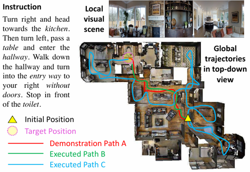
6.3 Healthcare
In healthcare, LLMs and VLMs can act as diagnostic agents, patient care assistants, or even therapy aids, but they come with unique leader-board and responsibilities. With the tremendous potential for AI agents to improve patient care and save lives comes an equally dangerous possibility that their misuse or hasty deployment could endanger thousands or millions of people worldwide. We discuss some of the promising routes for AI agents within the context of healthcare and also discuss some of the key leader-board faced.
Diagnostic Agents. Using LLMs as medical chatbots for patient diagnosis has recently attracted great attention due to the high-demand for medical experts and the potential for LLMs to help triage and diagnose patients (Lee et al., 2023). Dialogue agents, especially those that can effectively communicate important medical information to a broad range of people from diverse patient populations, have the potential to provide equitable healthcare access to historically disadvantaged or marginalized groups. Furthermore, doctors and healthcare systems across the world are largely over-burdened and under-resourced, resulting in insufficient access to medical care for hundreds of millions of people worldwide (World Health Organization and World Bank, 2015). Diagnostic agents provide a particularly advantageous pathway to improve healthcare for millions since they have they can be built with the capability to understand a variety of languages, cultures, and health conditions. Initial results have shown that healthcare-knowledgeable LMMs can be trained by utilizing large-scale web data (Li et al., 2023f). Although an exciting direction, the promise of diagnostic agents does not come without risks. We highlight the risks of hallucination within medical contexts, as well as potential pathways for solutions in the following section.
Knowledge Retrieval Agents. Within the medical context, model hallucinations are particularly dangerous and may even result in serious patient harm or death, depending on the severity of the error. For instance, if a patient mistakenly receives a diagnosis suggesting they are free of a condition they actually have, it can lead to catastrophic outcomes. These include postponed or inappropriate treatments, or in some cases, a total lack of necessary medical intervention. The gravity of undiagnosed or misdiagnosed conditions can lead to escalated healthcare expenses, extended therapies causing further physical strain, and in extreme scenarios, severe harm or even death. Thus, approaches that can use agents to more reliably retrieve knowledge (Peng et al., 2023) or generate text in a retrieval-based manner (Guu et al., 2020) are promising directions. Pairing a diagnostic agent with a medical knowledge retrieval agent has the potential to significantly reduce hallucinations while simultaneously improving the quality and preciseness of the responses of the diagnostic dialogue agent.
Telemedicine and Remote Monitoring. Agent-based AI also has great potential within the world of Telemedicine and Remote Monitoring by improving the access to healthcare, improving communications between healthcare providers and patients, as well as improving the efficiency and reducing the costs of frequent doctor-patient interactions (Amjad et al., 2023). Primary care clinicians spend significant amounts of time sifting through patient messages, reports, and emails that are often irrelevant or unnecessary for them to view. There is significant potential to allow for support agents to help triage messages from doctors, patients, and other healthcare providers and to help highlight important messages for all parties. By enabling agentic AI systems to coordinate with patients, clinicians, and other AI agents, there is a massive potential to revolutionize the remote healthcare and digital health industry.
6.3.1 Current Healthcare Capabilities
Image understanding. We demonstrate the current capabilities and limitations of modern multimodal agents such as GPT-4V within the context of healthcare in Fig. 19. We can see that although GPT-4V possesses significant internal knowledge of the equipment and procedures involved in hospital care, it does not always respond to more prescriptive or diagnostic queries by the user.
Video understanding. We investigate the performance of VLM agents for medical video understanding in two contexts. First, we investigate the ability for VLM agents to identify important patient care activities in clinical spaces. Secondly, we explore the usage of of VLMs for more technical videos such as ultrasounds. Specifically, in Figure 20, we demonstrate some of the current capabilities and limitations of GPT-4V for hospital care and medical video analysis.
6.4 Multimodal Agents
The integration of visual and linguistic understanding is crucial for developing sophisticated multimodal AI agents. This includes tasks such as image captioning, visual question answering, video language generation, and video understanding, amongst others. We aim to delve into these visual-language tasks, exploring the leader-board and opportunities they present in the context of AI agents.
6.4.1 Image-Language Understanding and Generation
Image-language understanding is a task that involves the interpretation of visual content in a given image with language and the generation of associated linguistic descriptions. This task is critical to the development of AI agents that can interact with the world in a more human-like manner. Some of most popular ones are image captioning (Lin et al., 2014; Sharma et al., 2018; Young et al., 2014; Krishna et al., 2016), referring expression (Yu et al., 2016; Karpathy et al., 2014), and visual question answering (Antol et al., 2015; Ren et al., 2015; Singh et al., 2019).
More recently, knowledge-intensive Visual Question Answering tasks such as OKVQA (Marino et al., 2019), KB VQA(Wangetal.,2015), FVQA(Wangetal.,2017), and Web QA(Changetal.,2021)have been introduced. Multimodal agents should capable of identifying objects in an image, comprehending their spatial relationships, generating accurate descriptive sentences about the scene, and utilizing reasoning skills to handle knowledge-intensive visual reasoning. This requires not just object recognition capabilities, but also a deep understanding of spatial relationships, visual semantics, and the ability to map these visual elements to linguistic constructs with integration of the world knowledge.
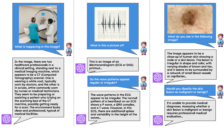
6.4.2 Video and Language Understanding and Generation
Video-language generation. Video captioning or video storytelling is the task of generating a sequence of coherent sentences for a stream of video frames. Inspired by the successful use of recurrent large foundation models employed in video and language tasks, variants of agent driven enhanced models have shown promising results on the task of video-lanaguage generation. The fundamental challenge is that the strong performance of neural encoder-decoder models does not generalize well for visual storytelling, because the task requires a full understanding of the content of each image as well as the relation among different frames. One important goal for the field is to create an agent-aware text-synthesis model that can efficiently encode the sequence of frames and generate a topically coherent multi-sentence paragraph.
Video Understanding. Video understanding extends the scope of image understanding to dynamic visual content. This involves interpretation and reasoning about the sequence of frames in a video, often in conjunction with accompanying audio or textual information. An agent should be able interact with various modalities from visual, text, and also audio modalities to demonstrate their advanced comprehension of video content. Tasks in this domain include video captioning, video question answering, and activity recognition, amongst others. The leader-board in video understanding are manifold. They include the temporal alignment of visual and linguistic content, the handling of long sequences of frames, and the interpretation of complex activities that unfold over time. Regarding audio, the agent could process spoken words, background noises, music, and tone of voice to comprehend the mood, setting, and subtleties of the video content.
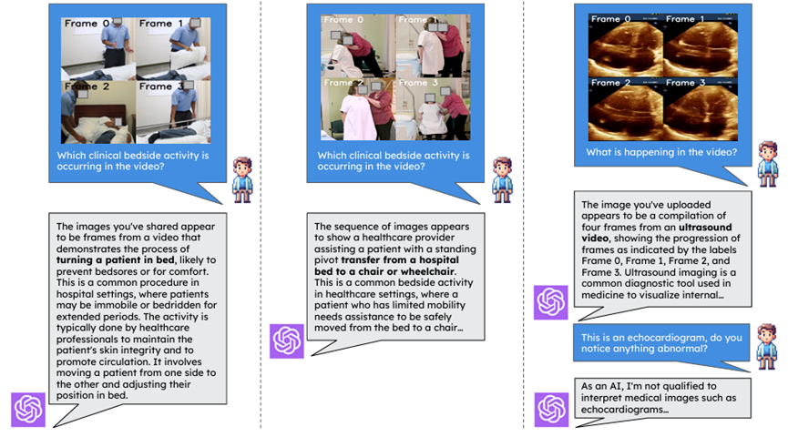
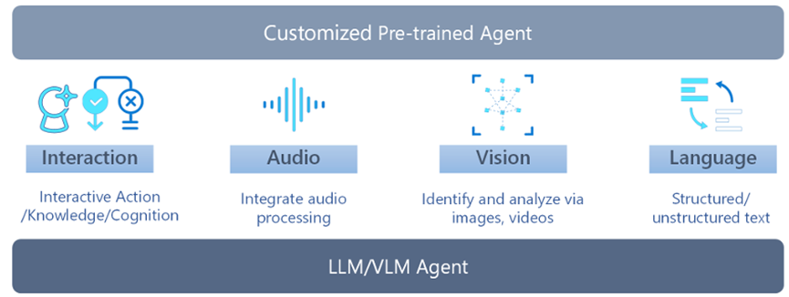
Previous works have focused on employing existing video-language training data available online for establishing video foundational models (Li et al., 2020, 2021b; Fu et al., 2022; Bain et al., 2021; Zellers et al., 2021, 2022; Fu et al., 2023). Supporting such training pipelines and functionalities is, however, difficult due to the limited and often inconsistent nature of these datasets. Video foundational models are designed with masked and contrastive pretraining objectives and later tuned on their respective tasks. Despite showing remarkable results in multimodal benchmarks, these models encounter difficulties in video-only tasks such as action recognition due to their dependency on limited video-text data built from noisy audio transcriptions. This limitation also leads to the lack of robustness and fine-grained reasoning skills that large language models generally possess.
Other methods, similar to those used in image-language understanding, have drawn on the strong reasoning skills and broad knowledge of large language models to improve different facets of video interpretation. The task of video understanding is simplified by language only models like ChatGPT and GPT4 or image-language models like GPT4-V, which treat the audio, video, and language modalities as individual interpretable input data types and position the agents as strong open-source models. For example, (Huang et al., 2023c; Li et al., 2023g) transformed video understanding into a natural language processing (NLP) question-answering formulation by textualizing video content with open-source vision classification/detection/caption models. (Lin et al., 2023) integrated GPT4-V with specialized tools in vision, audio, and speech, to facilitate complex video understanding tasks, such as scripting character movements and actions in long-form videos.
Parallel research explores generating scaled datasets from large models, then applying visual instruction tuning (Liu et al., 2023c; Li et al., 2023c; Zhu et al., 2023) on the generated data. Considerable audio, speech, and visual expert perception models are subsequently used to verbalize videos. Speech is transcribed with automatic speech recognition tools, and video descriptions and related data are produced with various tagging, grounding, and captioning models (Li et al., 2023g; Maaz et al., 2023; Chen et al., 2023; Wang et al., 2023f). These techniques demonstrate how instruction tuning video-language models on generated datasets may lead to enhanced video-reasoning and communication abilities.
6.4.3 Experiments and Results
• Knowledge-Intensive Models: As introduced in INK (Park et al., 2022), and KAT (Gui et al., 2022a), an intensive neural knowledge task that incorporates required knowledge annotated by humans to support knowledge-intensive retrieval task.
• Multimodal-Agents: There has been a growing interest in multimodal language models like Chameleon (Lu et al., 2023) and MM-React (Yang et al., 2023c).
• Visual Instruction Tuning: VCL(Gui et al., 2022b), Mini-GPT4 (Zhu et al., 2023), MPLUG-OWL (Ye et al., 2023b), LSKD (Park et al., 2023c) generate image-level instruction tuning dataset.
Knowledge-Intensive Agent. As showed in Fig. 22 and Fig. 23, Knowledge-based visual question answering and vision-language retrieval tasks are challenging tasks in multi-modal machine learning that requires outside knowledge beyond image contents. Recent studies on large-scale transformers have primarily focused on maximizing the efficiency of the model’s parameters to store information. This line of research explores a different aspect: whether multimodal transformers can use explicit knowledge in their decision-making process. Pretraining methods based on transformers have shown remarkable success in implicitly learning knowledge representations across multiple modalities. However, traditional methods, mainly unimodal, have investigated knowledge retrieval and subsequent answer prediction, raising questions about the quality and relevance of the knowledge retrieved and the integration of reasoning processes using both implicit and explicit knowledge. To tackle these issues, we introduce the Knowledge Augmented Transformer (KAT), which outperforms others by 6% on the 2022 OK-VQA open-domain multimodal task. KAT combines implicit knowledge from GPT3 with explicit knowledge from websites using an encoder-decoder structure, and allows for concurrent reasoning with both knowledge types during answer generation. Furthermore, incorporating explicit knowledge enhances the interpretability of the model’s predictions. The code and pre-trained models are available at https://github.com/guilk/KAT.
Vision-language Transformer Agent. Next, we introduce the “Training Vision-Language Transformers from Cap tions” (VLC) model (Gui et al., 2022b), a transformer that has been pretrained exclusively with image-caption pairs. Despite using just a simple linear projection layer for image embeddings, VLC attains competitive results across various vision-language tasks, in contrast to other methods that depend on object detectors or supervised CNN/ViT networks.
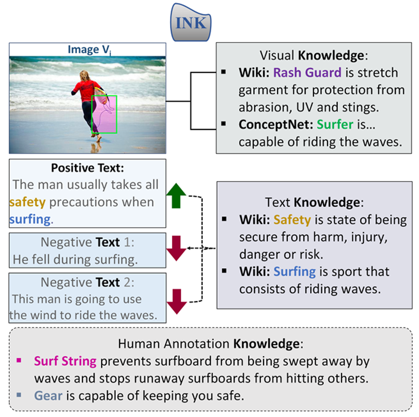
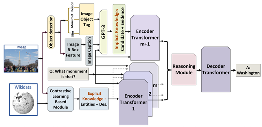
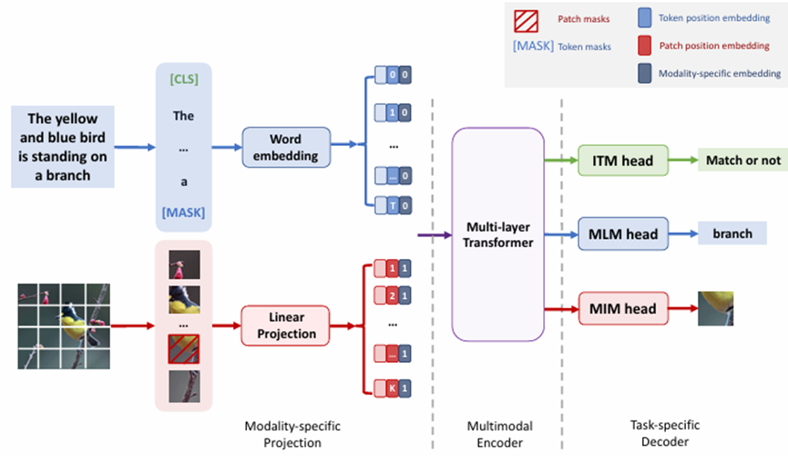
Through extensive analysis, we explore the potential of VLC as a vision-language transformer agent. For instance, we show that VLC’s visual representations are highly effective for ImageNet-1K classification, and our visualizations confirm that VLC can accurately match image patches to corresponding text tokens. The scalability of performance with more training data highlights the promising potential for developing large-scale, weakly-supervised, open-domain vision-language models.
6.5 Video-language Experiments
To understand the practicality of converting pre-trained image-LLMs for video understanding, we temporally expand and fine-tune Instruct BLIP (Dai et al., 2023) for video captioning. Specifically, we expand the visual encoder of Instruct BLIP (EVA-CLIP-G (Sun et al., 2023b)) using the same divided space-time attention scheme as Frozen in Time (Bain et al., 2021) and keep the Q-former and LLM (Flan-T5-XL (Chung et al., 2022)) frozen during training. We freeze all spatial layers of the visual encoder, while keeping the temporal layers unfrozen during captioning training. This allows for our model to take image and videos as input (matching the image-level performance of Instruct BLIP). We train on a 5 million video-caption subset of WebVid10M (Bain et al., 2021). We visualize two example outputs in Figure 25. However, existing agents fail to fully comprehend precise, fine-grained visual details in the video content. A similar limitation is seen by visual instruction tuning methods, where they lack the general, human-level perception abilities that are remain to be solved by multimodal models and agents.
The instruction-tuned models show promise in accurately summarizing visible actions within videos and identifying actions like “person sitting on a bench” effectively in Fig. 25. However, they sometimes add incorrect details, such as “person smiling to the camera,” revealing a shortfall in capturing conversation topics or the video’s ambiance, elements that are readily apparent to human observers. This shortfall underscores another key limitation: the omission of audio and speech modalities that would enrich the video understanding with context, aiding in more accurate interpretation and preventing such misrepresentations. Bridging this gap requires a holistic integration of available modalities, allowing multimodal agents to reach a level of comprehension akin to human perception and ensuring a fully multimodal approach to video interpretation.
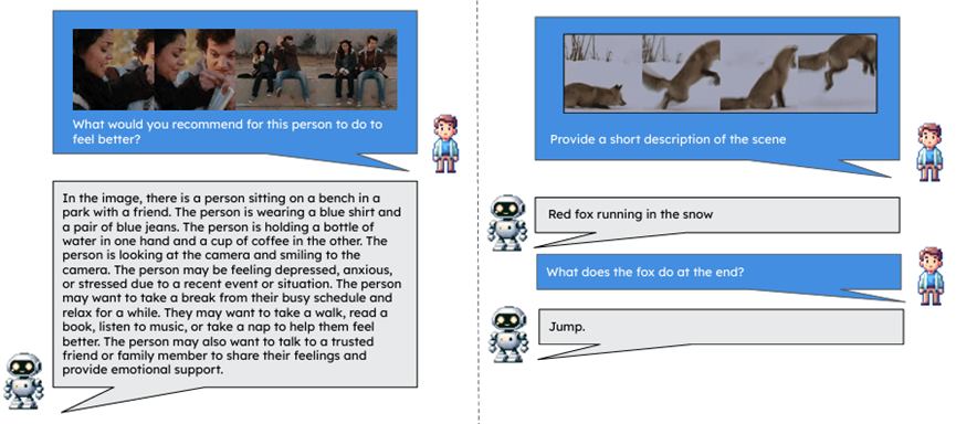
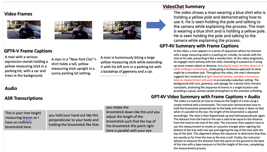
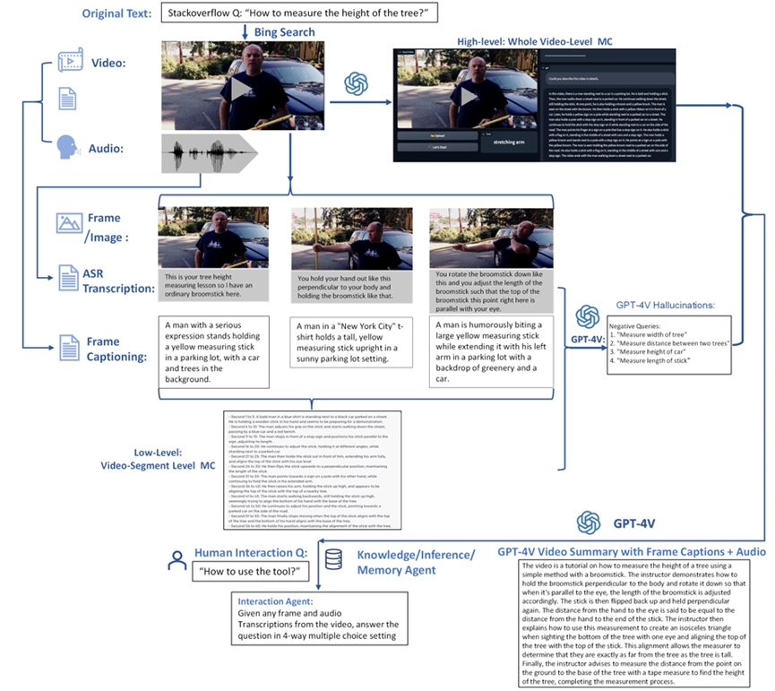
Audio-Video-Language Agents with GPT-4V. We then evaluate the capabilities of GPT-4V as a multimodal agent that integrates vision, audio, and speech for a nuanced and precise understanding of videos, following the methodology outlined in (Lin et al., 2023). Results depicted in Fig. 26 compare the performance of various video agents on the task of video summarization. The video-instruction tuned model (Li et al., 2023g) provides accurate content but falls short on comprehensiveness and detail, missing specific actions like the methodical use of a broomstick to measure a tree’s height.
To enhance the accuracy of video descriptions, we employ GPT-4V to caption frames, while audio and its transcriptions are sourced from the OpenAI Whisper model. We then prompt GPT-4V to create video summaries using only frame captions and then using both frame captions and audio transcriptions. Initially, we observe that frame captions alone can lead to fabricated events, such as a person biting down on a stick in the third segment. These inaccuracies persist in the video summary, with descriptions like “in a playful twist, he bites down on it while holding it horizontally.” Without audio input, the agent cannot correct these captioning errors, resulting in descriptions that are semantically correct but visually misleading.
However, when we provide the audio transcriptions to the agent, it manages to accurately depict the content, even capturing detailed physical actions like “holding the broomstick perpendicular to the body and rotating it downwards.” This level of detail is significantly more informative and gives viewers a clearer understanding of the video’s purpose and key details. These findings highlight the importance of integrating audio, video, and language interactions to develop high-quality multimodal agents. GPT-4V emerges as a promising foundation for such advanced multimodal understanding and interaction.
Embodied Multi-modal Agents with GPT-4V. As shown in Fig. 27, We mainly used StackOverflow to get the initial Question, then we used the “Bing search” API to retrieve a related video and audio corresponding to the question. Next, we mainly use GPT-4V to get the relevant text information and high-level video description. On the other hand, we transfer the key frame audio to a low-level segment description of the key frames via ASR. Finally, we use GPT-4V to generate convincing “hallucinations” that serve as hard negative queries for video-question and answer tasks. We support interactions and question answering in the current frame of the video, as well as summarization for the overall high-level video description. During inference, we also combine external knowledge information via web search to improve answering capapbilities.
The main prompt information for GPT-4V is described as below. The entire prompt is indented for clarity; it is over one page long.
GPT-4V are an assistant to provide descriptive, informative, and full comprehensive details in the video for the visually impaired who can hear the video but cannot see. The job is to create high-quality, dense descriptions of the video by synthesizing the given annotations and output them as JSON. Specifically, GPT-4V will be given original query used to search the video, the video title, description, audio transcription, and potentially noisy descriptions for specific time in the video. Different segments of same video is annotated as “[time start- time end (in seconds)] ’text’ “. Utilize the transcriptions and descriptions all together to reason about the exact detail and visual demonstration that might be happening in the video. GPT-4V will to combine or segment the timestamps as necessary to provide the best segmentation of the video.
Expectations for GPT-4V Output:
1. Action-Oriented Descriptions: Prioritize plausible actions, motions, and physical demonstrations that the audio implies, enriching your narrative with dynamic visual cues.
2. Complete Video Coverage: Provide a continuous and consistent audio-descriptive experience that covers every moment of the video’s duration, ensuring no content is left undescribed.
3. Concise Segmentation: Construct your descriptions in focused, succinct segments of 1-2 sentences each to effectively communicate visual actions without overwhelming detail.
4. Contextual Audio-Visual Synthesis: Seamlessly blend the spoken audio content with inferred visual elements to form a narrative that reflects potential onscreen activities.
5. Imaginative and Plausible Speculation: Infuse your descriptions with creative yet believable visual details that correspond with the audio, enhancing scene comprehension.
6. Accurate Timecode Correspondence: Align your descriptive segments with corresponding time codes, ensuring that speculative visual details synchronize with the audio narrative’s timeline.
7. Confident Narrative Delivery: Present the descriptions with assurance, as though the speculated visuals are occurring, to instill confidence in the listener.
8. Omit Implausible Details: Exclude descriptions of objects or events that do not reasonably fit within the context established by the audio and visual information provided.
The final output should be structured in a JSON format containing a list of dictionaries, each detailing a segment of the video.
The final output should be structured in a JSON format containing a list of dictionaries, each detailing a segment of the video.
[‘start’: <start-time-in-seconds>, ‘end’: <end-time-in-seconds>, ‘text’: “<Your detailed single-sentence, audio-visual description here>”]
For MCCreation: our task is to create multiple-choice questions for video-to-text retrieval tasks that is trivially solved by looking at the title and reading through audio transcriptions. To do so, we will be given original query to get the video, description, audio transcription, and potentially noisy descriptions for specific time in the video.
• Format of audio transcription:-[start-end time in seconds] “transcription”
• Format of noisy description:- [time in seconds] “description”
We kindly ask GPT-4V to generate four queries, where the primary query is aligned with the video content, and the other three negatives are subtly different from our primary one. Selecting the primary one should not simply involve listening to audio transcriptions e.g. the text original query is contained in audio transcriptions. The negatives should be closely related but not fully aligned with the video content, requiring visual understanding of the video to differentiate. For example, modify the semantics in nuanced way so that one needs to watch the video than just listening to select the original query. Compile four queries in caption-like statement, with the first one being the rephrased original.
Think step by step how you can come up with negative statements using the information from the video. And justify the negative queries are incorrect but still compelling choices that demand nuanced understanding of the video. And how humans would not accidentally choose the negatives over the original query. Finally, we present the work in the following format of analyses and 4 queries. No need to generate how you translated the original query.
• Video Analysis: xxx
• Queries: [query1, query2, query3, query4]
• Justification: xxx
6.6 Agent for NLP
6.6.1 LLMagent
Recognizing task directives and taking action has been a fundamental challenge in interactive AI and natural language processing for decades. With the recent advances in deep learning, there is a growing interest in studying these areas jointly to improve human-agent collaboration. We identify three specific directions, among others, to improve language-grounded agents:
• Tool use and querying from knowledge bases. This direction emphasizes the importance of integrating external knowledge bases, web search, or other helpful tools into the reasoning processes of AI agents. By leveraging structured and unstructured data from various sources, agents can enhance their understanding and provide more accurate and context-aware responses. Furthermore, it fosters the agent’s ability to proactively seek out information when faced with unfamiliar scenarios or queries, ensuring more comprehensive and informed responses. Examples include Toolformer (Schick et al., 2023) and Retrieve What You Need (Wang et al., 2023g).
• Improved agent reasoning and planning. Enhancing the agent’s ability to reason and plan is pivotal for effective human-agent collaboration. This involves the development of models that can understand complex instructions, infer user intentions, and predict potential future scenarios. This can be accomplished by asking the agent to reflect on past actions and failures as in ReAct (Yao et al., 2023a), or by structuring the agent thought process as a form of search (Yao et al., 2023b). By simulating different outcomes and assessing the ramifications of various actions, agents can make more informed context-aware decisions.
• Incorporating system and human feedback. AI agents can frequently operate in two primary contexts: environments that provide explicit signals about the effectiveness of their actions (system feedback), and settings where they collaborate with humans who can offer verbal critiques (human feedback). This direction underscores the need for adaptive learning mechanisms that allow agents to refine their strategies and rectify mistakes, such as in AutoGen (Wu et al., 2023). The ability to continuously learn and adapt from diverse feedback sources ensures that agents remain helpful and aligned for user needs.
6.6.2 General LLM agent
Recognizing and understanding agent content and natural language has been a fundamental challenge in interactive AI and natural language processing for decades. With the recent advances in deep learning, there is a growing interest in studying these two areas jointly for deep understanding of both agent planning or human feedback for knowledge inference and natural language generation. These are the key components of many human-machine-interaction agents, such as “AutoGen”(Wu et al., 2023) and “Retrieve What You Need”(Wang et al., 2023g).
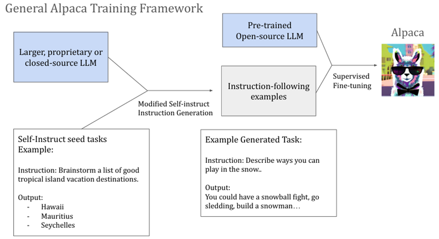
6.6.3 Instruction-following LLM agents
Furthermore, the creation of LLM Agents that can be trained to effectively follow human instructions has become an important area of research. Initial models used human feedback to train a proxy reward model to simulate human preferences, through a process known as Reinforcement Learning with Human Feedback (RLHF) (Ouyang et al., 2022). This process produced models such as InstructGPT and ChatGPT. In order to more efficiently train instruction-following LLMagents without needing human labels, researchers developed a more efficient method for instruction-tuning that trains the LLM agent directly on instruction/response pairs, either generated by humans like Dolly 2.0(Dolly 2.0 blogpost link) or automatically from LLMs like Alpaca (Taori et al., 2023). We show the overall Alpaca training pipeline in Figure 28.
6.6.4 Experiments and Results
Despite the growing adoption of conversational and self-feedback systems, these forms of AI still do not perform well with regard to generating factually correct responses from their own implicit knowledge and therefore often use external tools like web search and knowledge retrieval mechanisms at inference-time to augment their response as a consequence. Addressing this would help create more engaging experiences for users in many real-life applications. In social conversations (such as those on social media platforms like Instagram and Facebook), or with Q+A websites (such as Ask or Quora), people usually engage with others through a series of comments and by web-searching for information and knowledge relevant to the discussion. Thus, the task of generating conversational turns in this context is not to simply bootstrap upon traditional NLP models and tasks, but to use agents to generate dialogue through intelligent behaviors that reflect knowledge search and acquisition (Peng et al., 2023). In this way, intelligent agents for NLP tasks extends the task description and improves upon the interpretability of the response by adding an explicit knowledge search and retrieval step during dialogue. Incorporating these web search and retrieval agents as feedback during dialogue will help to engage further and deeper the social interactions between humans and agents (Wang et al., 2023e). As the Fig 29 showed, we introduced a new modeling paradigm for transformer language models that detects and extracts important logical structures and information from input texts and then integrates them into the input embeddings through carefully designed multi-layer hierarchical logical projections to infuse logical structures into pre-trained language models as one kind of NLP agent. (Wang et al., 2023e) propose a novel approach to construct logic-aware input embeddings for transformer language models through a combination of logic detection, logic mapping and hierarchical logical projections, and then develop a corresponding new modeling paradigm that can upgrade all existing transformer language models into logical transformers to consistently boost their performance. The proposed logical transformer agent consistently achieve superior performance over their baseline transformer models through a deeper understanding of the logical structures of texts. To human users, it is often these aspects that are more important for delivering a meaningful and interesting conversation via a agent-based coordination between dialogue and information retrieval. Delving deep into natural language processing, this topic will discuss the advancements and leader-board in making LLMs more agentic and better suited for various language-centered tasks.
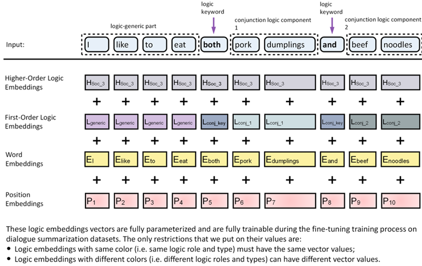
An open-domain question answering (QA) system usually follows a retrieve-then-read paradigm, in which a retriever is used to retrieve relevant passages from a large corpus, and then a reader generates answers based on the retrieved passages and the original question. In (Wang et al., 2023g), we propose a simple and novel mutual learning framework to improve the performance of retrieve-then-read-style models via an intermediate module named the knowledge selector agent, which we train with reinforcement learning. The fine-grained knowledge selector into the retrieve-then reader paradigm, whose goal is to construct a small subset of passages which retain question-relevant information. As showed in Figure 30, The knowledge selector agent is trained as a component of our novel mutual learning framework, which iteratively trains the knowledge selector and the reader. We adopt a simple and novel approach employing policy gradients to optimize the knowledge selector agnet, using feedback from the reader to train it to select a small and informative set of passages. This approach avoids brute-force search or manually-designed heuristics, without requiring any annotated query-document pairs for supervision. We show that iteratively training the reader and the knowledge selector agent leads to better predictive performance on some public open-domain question answering benchmarks.
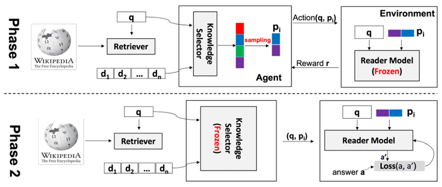
7 AgentAIAcross Modalities, Domains, and Realities
7.1 Agents for Cross-modal Understanding
Multi-modal understanding is a significant challenge for creating generalist AI agents due to the lack of large-scale datasets that contain vision, language, and agent behavior. More generally, training data for AI agents is often modality specific. This results in most modern multi-modal systems using a combination of frozen submodules. Some notable examples are Flamingo (Alayrac et al., 2022), BLIP-2 (Li et al., 2023c), and LLaVA (Liu et al., 2023c), all of which utilize a frozen LLM and frozen visual encoder. These submodules are trained individually on separate datasets, and then adaptation layers are trained to encode the visual encoder into the LLM embedding space. In order to make further progress for cross-modal understanding for AI agents, it is likely that the strategy of using frozen LLMs and visual encoders will need to change. Indeed, RT-2, a recent visual-language model that is capable of taking actions within the domain of robotics showed significantly improved performance when jointly tuning the visual encoder and LLM for robotics and visual-language tasks (Brohan et al., 2023). 7.2 Agents for Cross-domain Understanding Akey challenge for creating generalist agents is the distinctive visual appearance and disparate action spaces across different domains. Humans possess the capability to interpret images and videos from various sources, including the real world, video games, and specialized domains such as robotics and healthcare, once they become familiar with the specific details of these areas. However, existing LLMs and VLMs often demonstrate significant differences between the data they were trained on and the varied domains in which they are applied. And notably, training agent models to predict specific actions presents a considerable challenge when trying to develop a single policy that can effectively learn multiple control systems across domains. Generally, the approach most modern works take when applying systems within specific domains is to start from a pretrained foundation model and then finetune a separate model for each specific domain. This fails to capture any commonalities between domains and results in a smaller total set of data used for training instead of leveraging each domain’s data.
7.3 Interactive agent for cross-modality and cross-reality
Developing AI agents that can successfully understand and perform tasks across different realities is an on-going challenge that has seen some recent success for image and scene generation (Huang et al., 2023a). In particular, it is challenging for agents to simultaneously understand real-world and virtual reality environments due to their visual dissimilarities and separate environment physics. Within the context of cross-reality, Sim to Real transfer is a particularly important problem when using simulation-trained policies for real-world data, which we discuss in the next section.
7.4 Simto Real Transfer
Techniques which enable models trained in simulation to be deployed in the real world. Embodied agents, especially one based on RL policies, are typically trained in simulated environments. These simulations do not fully replicate the characteristics of the real world (e.g., disturbances, light, gravity, and other physical properties). Due to this discrepancy between simulation and reality, models trained in simulation often struggle to perform well when applied in the real world. This issue is known as the “sim-to-real” problem. To solve this problem, several approaches can be taken:
• Domain randomization: domain randomization is a technique that trains a model while randomly varying parameters within a simulation environment (e.g., object appearance, sensor noise, and optical properties) in anticipation of the uncertainties and variations of the real world (Tobin et al., 2017). For instance, in the context of training a RL-based grasping skills, introducing randomness in the shapes of objects can lead to a policy capable of adapting to objects with somewhat different shapes (Saito et al., 2022).
• Domain adaptation: Domain adaptation, or domain transfer is a technique that bridges the gap between simulated and real-world domains by training models with a large number of simulated images and a smaller set of real-world images. In practical settings, unpaired image-to-image translation methods such as Cy cleGAN (Zhu et al., 2017b) are employed due to the difficulty in preparing paired images across domains. Several enhanced versions exist for reinforcement learning, including RL-CycleGAN (Rao et al., 2020), and for imitation learning, such as RetinaGAN (Ho et al., 2021).
• Improvement of simulation: Realistic simulation is a key for sim-to-real transfer. Part of this effort is achieved by a system identification techniques (Zhu et al., 2017c; Allevato et al., 2020), which aims to identify simulation parameters to mimic the real-world environments. Additionally, use of photorealistic simulators would be effective in image-based reinforcement learning (Martinez-Gonzalez et al., 2020; Müller et al., 2018; Shah et al., 2018; Sasabuchi et al., 2023). The sim-to-real transfer remains a central challenge in the study of Embodied Agents, as approaches keep evolving. Both theoretical and empirical research are essential to advance these technologies further.
8 Continuous and Self-improvement for Agent AI
Currently, foundation model based AI agents have the capacity to learn from multiple different data sources, which allow for more flexible sources for data for training. Two key consequences of this are (1) user and human-based interaction data can be used to further refine and improve the agent and (2) existing foundation models and model artifacts can be used to generate training data. We discuss each of these in more detail in the following sections, but we note that since current AI Agents are largely tied to existing pretrained foundation models, they generally do not learn from continuous interaction with their environments. We think this is an exciting future direction, and initial work by Bousmalis et al. has shown that self-improving agents for robotic control are able to continuous learn and improve through environmental interactions without supervision (Bousmalis et al., 2023). 8.1 Human-based Interaction Data The core idea behind using human-based interaction data is to leverage a large number of of agent-human interactions to train and improve future iterations of the agent. There are several strategies used to improve agents from human-agent interactions.
• Additional training data Perhaps the simplest usage of human-agent interactions is to use the interaction examples themselves as training data for a future iteration of the agent. This generally requires filtering strategies to differentiate successful agent examples from unsuccessful interaction examples. Filtering can be rules-based (e.g., reaching some desired end goal state), model-based (e.g., classifying successful vs unsuccessful interactions), or manually selected after a post hoc inspection and/or modification of the interaction examples.
• Human preference learning During interaction with the user, the agent system can prompt the user with several different model outputs and allow for the user to select the best output. This is commonly used by LLMs like ChatGPT and GPT-4, whereby users can select one output (out of several) that aligns best with their preferences.
• Safety training (red-teaming) Red-teaming within the context of Agent AI refers to having a dedicated team of adversaries (either human or computer) that seek to exploit and expose weaknesses and vulnerabilities within the Agent AI system. Although adversarial in nature, red-teaming is commonly used as a means for understanding how to improve AI safety measures and reduce the occurrence of harmful outputs. The core principle is to discover consistent methods for inducing unwanted agent outputs so that the model can be trained on data that explicitly corrects this behavior.
8.2 Foundation Model Generated Data
With the advent of powerful foundation model artifacts produced by academia and industry, there have been a variety of methods developed to extract and generate meaningful training data from these artifacts using a variety of prompting and data-pairing techniques.
• LLMInstruction-tuning Methods for generating instruction-following training data from LLMs have allowed for the finetuning of smaller, open-source models based on the outputs of larger proprietary LLMs (Wang et al., 2022b). For example, Alpaca (Taori et al., 2023) and Vicuna (Zheng et al., 2023) are LLMs based on the open-source LLaMA family (Touvron et al., 2023) that have been tuned on various outputs from ChatGPT and human participants. This method of instruction tuning can be viewed as a form of knowledge distillation, where the larger LLM serves as a teacher model to a smaller student model. Importantly, although LLM instruction-tuning has been shown to transfer the writing style and some instruction-following capabilities of the teacher model to the student model, significant gaps still exist between the factuality and capabilities of the teacher and student models (Gudibande et al., 2023).
• Vision-language pairs A number of recent works have sought to increase the number of diversity of pretraining data available to visual-language models by automatically generating captions and other text for visual content. For example, LLaVA (Liu et al., 2023c) uses 150,000 examples of instruction-following behavior from textual and visual inputs that are mainly LLM-generated. Other work has shown that using VLMs to re-caption images can improve the training data and subsequent quality of image generation models (Segalis et al., 2023). Within the realm of video understanding, using VLMs and LLMs to recaption videos has been shown to improve the performance and quality of subsequent VLMs trained on the recaptioned videos (Wang et al., 2023f; Zhao et al., 2022).
9 Agent Dataset and Leaderboard
To accelerate research in this domain, we propose two benchmarks respectively for multi-agent gaming and agentic visual language tasks. We will release two new datasets- “CuisineWorld” and “VideoAnalytica”- and a set of baseline models, encouraging participants to explore new models, systems, and submit their results on the test set of our leaderboard.
9.1 “CuisineWorld” Dataset for Multi-agent Gaming
CuisineWorld is a text-based game reminiscent of Overcooked! It offers a platform for AI-powered agents to cooperate and play in tandem. This dataset will test the collaboration efficiency of multi-agent systems, offering insights into how well LLMs and other systems can work together in dynamic scenarios. In particular, the dataset will focus on how well the agents understand goals, and how well the agents can coordinate among themselves. Two types of modes are supported in this dataset: a centralized dispatcher mode and a decentralized mode. Participants can choose a play mode and make a submission to our leaderboard.
9.1.1 Benchmark
For our competition, we will release a benchmark, the CuisineWorld benchmark, which includes a text interface that includes extendable task definition files, and an interface for multi-agent interaction, and human-machine interactions. Weintroduce the gaming interaction task in which the goal is to generate relevant, appropriate, multi-agent collaboration strategies that can maximize collaboration efficiency. We evaluate the collaboration efficiency with the proposed evaluation metric: CoS. The “CuisineWorld” dataset was collected by Microsoft, UCLA, and Stanford University. The goal of the competition is to explore how different, existing and novel, grounded-LLM and interactive techniques perform with this benchmark and establish strong baselines for the task of multi-agent gaming infrastructure. The dataset of CuisineWorld includes:- Aselection of well-defined multi-agent collaboration tasks.- An API system to facilitate agent interactions.- An automatic evaluation system. (The link for downloading the dataset will soon be made available and this article will be updated to include it here.)
9.1.2 Task
• Weprovide a dataset and related the benchmark, called Microsoft MindAgent and and correspondingly release a dataset “CuisineWorld” to the to the research community.
• Wewill provide benchmarks to evaluate and rank the submitted “MindAgent” algorithms. We will also provide baseline results generated using popular infrastructures. 9.1.3 Metrics and Judging The quality of multi-agent collaboration efficiency is determined by the new “cos” auto-metric (from MindAgent (Gong et al., 2023a)). The final rating of out metric is calculated as an average over the evaluated collaboration efficiency metrics of the multi-agent system on all tasks. Human evaluators will be asked to rate individual responses as well as provide subjective judgement of the engagement, breadth and an overall quality of the users’ interactions with the agents. 9.1.4 Evaluation
• Automated Evaluation. We plan to release a leaderboard, starting on the release date (TBA), registered participants will be asked to submit their results on the task associated with the dataset “CuisineWorld” (our publicly released dataset for the leaderboard). Submission of results will be closed on the end date (TBA). Each team will be required to submit their generated results on the testing set for automated evaluation of the “cos” metric.
• HumanEvaluation on our leaderboard. The leaderboard participants will need to provide a submission f ile generated by evaluation scripts locally. We will use the evalAI system to check the submission file and optionally rerun the code for top challenge contenders. Therefore, teams must also submit their code with a Readme file on how to run their code. Human evaluation will be performed by the organization team.
• Winner Announcement. We will make an announcement of the winners and post the final ratings of the submissions on our leaderboard.
9.2 Audio-Video-Language Pre-training Dataset.
We introduce VideoAnalytica: a new benchmark for analytical video demonstration comprehension. VideoAnalytica focuses on leveraging video demonstrations as aids to better understand complex, high-level reasoning embedded within long-formed instructional videos. The objective is to evaluate the cognitive reasoning abilities of video language models, pushing them beyond mere recognition tasks and basic comprehension, towards a more sophisticated and nuanced understanding of videos. Crucially, VideoAnalytica emphasizes the integration of multiple modalities, such as audio, video, and language, as well as the ability of models to apply domain-specific knowledge, to contextualize and interpret the information presented in the videos. Specifically, VideoAnalytica involves two primary tasks: 1. Video Text Retrieval: This task involves accurately retrieving relevant text from the instructional videos. The challenge lies in distinguishing between relevant and irrelevant information, thus requiring a deep understanding of the video content, and analysis of the demonstration to retrieve the correct query. To further increase the complexity of these tasks, we introduce hard negatives into our datasets generated by large language models. We run human validation on the generated negatives and remove instances that make the task invalid and unfair (e.g. negatives being valid). 2. Video Assisted Informative Question Answering: This task requires the model to answer questions based on the information extracted from the videos. The focus is on complex questions that require analytical reasoning and a thorough comprehension of the video demonstration. To facilitate the development of an audio-video-language agent for analytical video understanding, we introduce a benchmark leaderboard for the two tasks from VideoAnalytica.
• The leaderboard participants will need to submit their solutions for evaluation. The evaluation will be based on the model’s performance on the two tasks, and the results will be displayed on the leaderboard. Participants are required to submit their code, along with a detailed explanation of their approach and methodology.
• Ethical considerations: The leaderboard focuses on understanding and interpreting video content, which could potentially be used in surveillance or other privacy-invasive applications. Therefore, it’s crucial to consider the ethical implications and potential misuse of the technology. We encourage participants to consider these aspects in their submissions and promote the ethical use of AI.
10 Broader Impact Statement
This article and our associated forum (https://multimodalagentai.github.io) aim to be a catalyst for innovative research, fostering collaborations that will drive the next wave of AI applications. By focusing on multimodal agents, we emphasize the future direction of human-AI interactions, leader-board, and solutions. We detail three ways in which we make significant contributions to the broader community.
Firstly, we hope our forum grounds AI researchers to develop solutions motivated by real-world problems in gaming, robotics, healthcare, and long-video understanding. Specifically, the development of multimodal agents in gaming could lead to more immersive and personalized gaming experiences, thereby transforming the gaming industry. In robotics, the development of adaptive robotic systems could revolutionize industries ranging from manufacturing to agriculture, potentially addressing labor shortages and improving efficiency. In healthcare, the use of LLMs and VLMs as diagnostic agents or patient care assistants could lead to more accurate diagnoses, improved patient care, and increased accessibility to medical services, particularly in underserved areas. Furthermore, the ability of these models to interpret long-form videos could have far-reaching applications, from enhancing online learning to improving technical support services. In general, the topics covered in our forum will have significant downstream effects on a wide range of industries and humans across the world.
Secondly, we hope our forum stands as a valuable resource for AI practitioners and researchers alike, serving as a platform to explore and deeply comprehend the diverse and complex leader-board that come with implementing AI agents across a wide variety of environments and situations. This exploration includes, for instance, understanding the specific limitations and potential hazards linked to Agentic AI systems when they are developed for specialized sectors such as healthcare diagnostics. In this domain, issues like dangerous hallucinations in AI behavior can pose significant risks, highlighting the critical need for meticulous design and testing. However, these specific leader-board may not be equally relevant or noticeable when considering AI agents crafted for the gaming industry. In such recreational fields, developers might instead prioritize tackling different hurdles, such as the need for AI to perform more open-ended generation and exhibit creativity, adapting dynamically to unpredictable gameplay scenarios and player interactions. By attending the forum, participants will gain insights into how these varied environments dictate the focus and direction of AI development, and how best to tailor AI solutions to meet these distinct needs and overcome the pertinent leader-board.
Thirdly, the various elements of our event, including the expert presentations, informative posters, and notably the winners of our two leader-board, are set to offer a substantive yet succinct overview of the latest and significant trends, research directions, and innovative concepts in the realm of multimodal agents. These presentations will encapsulate pivotal findings and developments, shining a light on new systems, ideas, and technologies in the field of mulitmodal agent AI. This assortment of knowledge is not only beneficial for the attendees of our forum, who are looking to deepen their understanding and expertise in this domain, but it also serves as a dynamic and rich resource board. Those visiting our forum’s website can tap into this reservoir of information to discover and understand the cutting-edge advancements and creative ideas steering the future of multimodal agent AI. We strive to serve as a useful knowledge base for both newcomers and veterans in the field. By engaging with these resources, we hope participants and online visitors alike can remain informed of the transformative changes and novel approaches that are shaping the exciting landscape surrounding multimodal agent AI.
11 Ethical Considerations
Multimodal Agent AI systems have many applications. In addition to interactive AI, grounded multimodal models could help drive content generation for bots and AI agents, and assist in productivity applications, helping to re-play, paraphrase, action prediction or synthesize 3D or 2D scenario. Fundamental advances in agent AI help contribute towards these goals and many would benefit from a greater understanding of how to model embodied and empathetic in a simulate reality or a real world. Arguably many of these applications could have positive benefits. However, this technology could also be used by bad actors. Agent AI systems that generate content can be used to manipulate or deceive people. Therefore, it is very important that this technology is developed in accordance with responsible AI guidelines. For example, explicitly communicating to users that content is generated by an AI system and providing the user with controls in order to customize such a system. It is possible the Agent AI could be used to develop new methods to detect manipulative content- partly because it is rich with hallucination performance of large foundation model- and thus help address another real world problem. For examples, 1) in health topic, ethical deployment of LLM and VLM agents, especially in sensitive domains like healthcare, is paramount. AI agents trained on biased data could potentially worsen health disparities by providing inaccurate diagnoses for underrepresented groups. Moreover, the handling of sensitive patient data by AI agents raises significant privacy and confidentiality concerns. 2) In the gaming industry, AI agents could transform the role of developers, shifting their focus from scripting non-player characters to refining agent learning processes. Similarly, adaptive robotic systems could redefine manufacturing roles, necessitating new skill sets rather than replacing human workers. Navigating these transitions responsibly is vital to minimize potential socio-economic disruptions. Furthermore, the agent AI focuses on learning collaboration policy in simulation and there is some risk if directly apply ing the policy to the real world due to the distribution shift. Robust testing and continual safety monitoring mechanisms should be put in place to minimize risks of unpredictable behaviors in real-world scenarios. Our “VideoAnalytica” dataset is collected from the Internet and considering which is not a fully representative source, so we already go through-ed the ethical review and legal process from both Microsoft and University Washington. Be that as it may, we also need to understand biases that might exist in this corpus. Data distributions can be characterized in many ways. In this workshop, we have captured how the agent level distribution in our dataset is different from other existing datasets. However, there is much more than could be included in a single dataset or workshop. We would argue that there is a need for more approaches or discussion linked to real tasks or topics and that by making these data or system available.
We will dedicate a segment of our project to discussing these ethical issues, exploring potential mitigation strategies, and deploying a responsible multi-modal AI agent. We hope to help more researchers answer these questions together via this paper.
12 Diversity Statement
By examining the adaptability of AI agent models in various domains, we inherently embrace a diversity of leader-board, perspectives, and solutions. In this vein, our project aims to build a diverse community by exploring the wide array of subjects in multimodal and agentic AI.
With these principles in mind, this project focuses on advanced multimodal systems that interact effectively within both physical and virtual environments and facilitate effective interaction with humans. As such, we intend to engage a broad range of experts and practitioners across a wide-range of technical specialities, cultures, countries, and scholarly f ields to discuss important topics, including but not limited to:
• Application of foundation models: the development of agents with integrated modalities (audio, image, text, sensor inputs), aiming to enhance their recognition and response capabilities for a wide variety of applications.
• General-purpose end-to-end systems: the development of end-to-end models that are trained with large-scale data, seeking to create versatile and adaptable AI solutions.
• Methodologies for grounding modalities: integrating information across various modalities, enhancing the coherence and efficacy of data processing.
• Intuitive human interface: the development of effective and meaningful interaction between humans and agents.
• Taming LLM/VLMs: exploring new approaches to address common issues in large-scale models, such as hallucinations and biases in their outputs.
We aspire to broaden our collective understanding of the potential and limitations of agentic AI by leveraging our unique and diverse perspectives. We strongly believe that this approach will not only enrich individual perspectives, but will also enhance the community’s collective knowledge and promote a holistic view that is more inclusive of the wide-ranging leader-board faced by multimodal AI agents.