作者: deepoo
-
余少祥:论社会法的本质属性[节]
一、体现社会法本质的基本范畴
范畴及其体系是衡量人类在一定历史时期理论发展水平的指标,也是一门学科成熟的重要标志。社会法的基本范畴是社会法的概念、性质及结构体系等内容的本质体现,这是当前学术界研究相对薄弱的环节。社会法的基本范畴经历了从社会保护、社会保障到社会促进,从生存性公平到体面性公平的演变,体现了社会法不同于其他部门法的本质特征。
(一)国内立法史视角
一直以来,我国社会法的基本范畴都是社会保护,主要体现为对特定弱势群体的生活救济和救助。到了近代,开始探索社会保障制度。新中国成立尤其是新时代以来,社会促进逐渐成为社会法的新追求。
在我国古代,虽然没有系统的社会法制度体系,但很早就有关于社会救济的思想和行为记载,如《礼记·礼运》提出“使老有所终,壮有所用,幼有所长,鳏寡孤独废疾者,皆有所养”;《墨子》主张“饥者得食,寒者得衣,劳者得息”。在制度方面,《礼记·王制》言及夏、商、周各代对聋、哑等残障人士“各以其器食之”。在西周,六官中地官之下设大司徒,专门负责灾害救济。春秋战国时期,增加了“平籴、通籴”等措施。两宋之后,居养机构发展较为完善,有福田院、居养院等多种形式。此外,还有用于赈灾的名目众多的仓储体系,如汉有常平仓,唐有义仓,两宋有惠民仓、社仓,元有在京诸仓、御河诸仓,明有预备仓等。但总体上看,这些救助措施均非法定义务。统治者赈灾济困乃是一种怀柔之术,是为巩固皇权的收买人心之举,与现代意义的社会法相距甚远。
我国真正开启社会立法的是北洋政府。清末搞得沸沸扬扬的修宪和制订法律的活动,催生了民法、刑法等一批法律法规,却没有一部关于社会救济和保障民众生活的法律。1923年,北洋政府颁布《矿工待遇规定》,首次引入“劳动保险”概念,可谓我国社会法的破壳之作。可惜,这些法令因战乱和时局动荡刚实施便很快夭折。南京国民政府建立后,先后颁布《慈善团体监督法》《救灾准备金法》《最低工资法》等。从抗日战争起,以国民政府社会部成立为标志,社会立法渐趋完备。1943年《社会救济法》颁布,奠定了民国社会法的基石。这一时期,《社会保险法原则》《职工福利社设立办法》等先后公布,为探索社会保障进行了有益尝试,社会法发展开始迈入现代化门槛。但由于内战不断、政局不稳、政令不畅,加上官僚买办资本的抵制,这些法令并没有得到有效实施。
新中国成立后,我国实行的是计划经济体制和单位对职工生老病死全包的政策。直到20世纪80年代,民众的基本生活保障仍是由国家和集体组织承担。90年代起,随着向市场经济转型,一部分群体开始从单位人向“社会人”转变。为确保这部分民众的基本生活来源,我国开始建立社会保障制度,先后颁布《残疾人保障法》(1990)、《劳动法》(1994)、《城市居民最低生活保障条例》(1999)等社会法规。进入21世纪后,相继出台了《劳动合同法》(2007)、《社会保险法》(2010)等社会立法。新时代以来,又陆续推出《慈善法》(2016)、《法律援助法》(2021)等,加上之前的《红十字会法》(1993)、《就业促进法》(2007),社会促进逐渐成为立法的关键词。从总体上看,我国当代社会立法是制度变迁的产物,而非在市场发展中形成的,因此与西方国家有所不同。
(二)国外立法史视角
社会法是舶来品,深受欧美日等工业国家影响,因此探求社会法的概念、范畴与体系等,离不开对外国法制的比较观察。从总体上看,国外社会法范畴也经历了社会保护、社会保障和社会促进的演进。
英国是世界上最早实行社会立法的国家,其目的是为脆弱群体提供社会保护。1388 年,金雀花王朝制定了一部《济贫法案》。1531年,亨利八世又颁布了一部《名副其实救济法》,规定老人和缺乏能力者可以乞讨,地方当局将根据良心从事济贫活动。这两个法案与1601年伊丽莎白《济贫法》相比,影响较小。后者诞生于“羊吃人”的圈地运动时期,旨在“将不附任何歧视性的工作给有工作能力的人”,后为很多国家效仿。1563年,英国颁布了历史上第一部《劳工法》,1802—1833年又颁布5个劳动法案,覆盖了几乎所有工业部门,确立了现代劳动保护体系及基本原则。1834年,英国政府出台《济贫法修正案》,史称“新济贫法”。这些立法孕育着社会法的丰富遗产,具有鲜明的时代性、体系性和结构性特征。此后欧洲其他工业化国家纷纷仿效英国,建立起自己的社会保护制度。
世界上最早实行社会保险立法的是德国。19世纪中后期,俾斯麦政府采取“胡萝卜加大棒”政策,一面对工人阶级反抗实施残酷镇压,一面通过社会保险对其安抚,相继出台了《疾病保险法》(1883)、《工伤保险法》(1884)等法规。由于社会保险法适应了工业化对劳动力自由流动的需求,解决了劳动者生活的后顾之忧,在社会法体系中占有重要地位。但西方社会法真正完成的标志是1935年美国《社会保障法》施行,这是社会保障概念在世界上首次出现。之后,社会法的发展开始进入一个新的历史阶段——为社会成员提供普遍福利,其典型标志是英国“贝弗里奇计划”实施。由于该计划被逐步纳入立法,标志着英国社会法走向完备和成熟。第二次世界大战后西方各国在推行社会立法时,不同程度借鉴了《贝弗里奇报告》模式,使得西方社会法的福利化转型最终完成。
20世纪60年代,西方国家普遍解决了生存权问题,社会促进开始成为立法的重要权衡。除了传统的慈善法大量兴起外,扶贫法和反歧视法逐渐形成新的热潮。以美国为例,1964年约翰逊政府通过《经济机会法》,宣布“向贫困宣战”,此外还实施了社区行动计划、学前儿童启蒙教育计划等。其他国家如英国的《儿童扶贫法案》、法国的“扶贫计划”和德国的《联邦改善区域结构共同任务法》等在促进落后地区经济社会发展方面也起到了重要作用。在反歧视方面,美国、英国、欧盟和日本都有完备的立法。尤其是美国,仅反就业歧视法就多达十余部,且有大量判例具有重要立法价值。这一时期,日本的《反对性别歧视法》(1975)、瑞典的《男女机会均等法》(1980)等纷纷出台。根据反歧视法的差别待遇原则,都是为了促进国民获得实际平等地位,实现社会实质公平。
(三)学术研究史视角
我国社会法研究肇始于民国初期。1949年以后,又分为“大陆”和“台湾地区”两个支系,前者的探索早于后者,而且在一定程度上沿袭了民国的传统。从学术史上看,学术界在某些观点上取得了较大共识,但核心范畴略有差异。
民国的社会保护和社会幸福说。多数民国学者认为,社会法是救济和保护社会弱者之法。如李景禧提出,社会法是“为防止经济弱者地位的日下,调整了暂时的矛盾”。陆季藩指出,社会法是“以保护劳动阶级或社会弱者为目标”的法。林东海认为,凡是“解决社会上之经济的不平等问题”的立法,都是社会法。杨智提出,社会法是“以增进及保护社会弱者之利益为目的”的法。也有学者主张,社会法包含一般社会福利。如张蔚然提出,社会法是“关于国民经济生活之法”。卢峻认为,社会法的目标是“使社会互动关系或社会连立关系”达到最高目标。黄公觉则明确提出,广义社会法“指一切关于促进社会幸福的立法”,狭义社会法仅指“为促进社会里的弱者或比较不幸者的利益或幸福之立法”。
大陆的劳动保护与社会保障说。1993年,中国社会科学院法学研究所在一份报告中将社会法解释为“调整因维护劳动权利、救助待业者而产生的各种社会关系的法律规范的总称”。这是新中国学术界首次系统阐述这一概念。最高人民法院2002年编纂的《社会法卷》认为,“坚持社会公平、维护社会公共利益、保护弱势群体的合法权益”是“社会法的主要特点”。在学术界,多数学者将社会法定义为调整劳动与社会保障关系的法律。如张守文认为,社会法“具有突出的保障性”,主要是“防范和化解社会风险和社会危机,保障社会安全和社会秩序”;赵震江等认为,社会法是“从整个社会利益出发,保护劳动者,维护社会稳定”,包括“社会救济法、社会保障法和劳动法等”。从中国社会法学研究会历次年会讨论的情况来看,劳动法、社会保障法、慈善法属于社会法的观点已被普遍接受。
台湾地区的社会安全和生活安全说。很多台湾学者从社会保护出发,将社会法称为社会安全法。如王泽鉴认为,社会法“系以社会安全立法为主轴所展开的”。钟秉正认为,社会法是“以社会公平与社会安全为目的之法律”,“以消除现代工业社会所产生的各种不公平现象”。也有学者明确提出社会法是生活安全法。如郝凤鸣认为,社会法是“以解决与经济生活相关之社会问题为主要目的”,“藉以安定社会并修正经济发展所造成的负面影响”;陈国钧认为,社会法旨在保护某些特殊人群的“经济生活安全”,或用以促进“社会普遍福利”,这些法规的集合被称为社会法或社会立法。总之,在台湾学术界,社会法集中指向与社会保护、社会保障和社会福利等相关的社会安全或生活安全法。
二、决定社会法本质的要素分析
事物的本质和发展方向是由核心要素决定的,在讨论社会法的本质之前,我们先分析决定其本质的核心要素。如前所述,社会法产生的根源是社会的结构性矛盾,尤其是市场化带来诸多社会问题,使得国家不得不运用公权力干预私人经济,达到保障民众生存权、化解社会矛盾的目的。在一定意义上,政治国家、经济社会和历史文化等要素在社会法本质形成过程中起到了决定性作用。
(一)政治国家要素
作为国家在干预私人领域过程中形成的全新法律门类,社会法与传统的自由权、自由市场经济体制以及民主法治国家理念存在一定冲突。正是国家职能的转变决定了社会法的内在精神和本质,使人民受益于国家的关照。
1.从消极国家到积极国家
在古典自由主义时期,政府主要承担“守夜人”角色。资本主义发展到垄断阶段以后,不但造成市场机制失灵,而且难以维持社会稳定。于是,社会上层开始形成一种共识,即通过国家干预,改良资本主义制度,以消除暴力革命的隐患。正如马克思和恩格斯指出,“资产阶级中的一部分人想要消除社会弊病”,“但是不要由这些条件必然产生的斗争和危险”。按照黑格尔的阐述,国家的目的在于“谋公民的幸福”,否则它“就会站不住脚的”。在这种情形下,国家这只“看得见的手”开始不断发挥作用,以平衡不同社会群体的需求,积极国家随之诞生。因此,国家干预并非理论家的发明,而是在历史进程中实际发生的,即对抗已重新采取直接的国家干涉主义形式,国家进一步成为社会秩序的干预者。
国家干预社会生活是通过社会立法实现的,直接决定了社会法的性质和宗旨。由于国家不得不采取干涉主义的社会立法来做社会救济的工具,于是在法律上体现为,国家对于任何人都有保障其基本生活的义务。从立法宗旨来看,旨在打破弱肉强食的丛林法则,将社会贫富分化控制在一个可以承受的动态合理范围之内。比如,通过劳资立法,克服自由资本主义无节制地追求高额利润造成的社会分裂等严重后果。事实上,国家实行经济社会干预,不是否认私人利益和个人需求,而是将其重整到更高的全社会层面,即运用国家的力量实现个人的特殊利益与社会整体利益的统一。因此,社会法表面上是社会性的,实质上是政治性的,是一种典型的政治法学,它发轫于人对国家的依附性,发生于国家对共同体内每个人的幸福所负有的法律责任,使国民的生活安全得到有效保障。
2.从社会国到福利国家
积极国家进一步引发从消极自由到积极自由的发展。也就是说,国家不仅有保障公民基本自由不受侵犯的消极义务,更有保障公民基本生存与安全的积极义务,这也是社会发展进步的重要标志。在这一背景下,政府不再像以前一样仅仅囿于维护社会秩序,或对出现的问题进行决策干预,而是更进一步转换为保障人民具有人格尊严和最低生存条件的给付行政。通过给付行政,政府承担了涵盖广泛的计划性的行为、社会救济与社会保障等任务。尤其是在工业社会条件下,国民享有基本权利和事实自由的物质基础并不在于他们为社会作过什么贡献,而根本上依赖于政府的社会给付。正是给付行政成就了今天的社会国,即一个关照社会安全与民生福祉的国家。社会法便是为实现社会国的目标任务形成的法律体系,而社会国原则又为立法者干预私人领域提供了合法性依据。
19世纪末20世纪初,随着垄断资本主义发展,社会本位的法理念开始取代个人本位的法思想并居于支配地位。这一时期,政治国家与市民社会的矛盾在法律上体现的结构也发生了新变化,使得国家在向国民承诺下不断增加福利范围。1942年,英国“贝弗里奇计划”首次采用福利国家称谓,通过财产重新配置,为公民提供基本生活保障。二战之后,这一思想主宰了西方的正统观念,很多国家确认促进民生幸福是公民的重要社会权利,对广泛和普遍的社会福利而言同样如此,国家承担了民众直接或间接的生活责任。可见,政治国家不但有力地推动了社会法的发展,而且决定了其福利化方向,最大限度地消除了各阶级之间的对抗冲突以及社会革命的危险,促进了社会公正公平,有效维护了社会稳定。
(二)经济社会要素
工业革命以后,资本主义的新信念是唯物质主义的,即只要物质财富足够多,一切社会问题都会自动消失。事实上,纯粹的市场机制无法解决社会公平、效率以及经济长期稳定等重要问题。由于市场体系造成了巨大的社会混乱,如果不深刻调整,市场机制也将被摧毁。因此,资产阶级国家被迫用法律来防止资本主义剥削过度的现象,通过社会立法去收拾资本和市场留下的烂摊子,出现了以社会法为核心、旨在对冲和矫治市场化不利后果的社会保护运动,结果连最纯正的自由主义者也承认,自由市场的存在并不排斥对政府干预的需要。正如罗斯福在1938年向国会提交的一份“建议”中指出:“我们奉行的生活方式要求政治民主和以营利为目的的私人自由经营应该互相服务、互相保护——以保证全体而不是少数人最大程度的自由。”
经济民主理论认为,经济问题与伦理问题密切相关,人类经济生活应满足高尚、完善的伦理道德方面的欲望。社会法倡导社会保险、社会救济、劳工保护等社会权利,以解决资本主义发展中日益严峻的社会问题。一方面,要保障每个人拥有获取扩展其能力的物质条件和自我实现的机会;另一方面,要在支持扩大国家给付的理由与加重政府财政负担的结果之间进行权衡。可见,社会法的产生不单纯是对民众生活的保护,也是产业制度有效运行和社会存续的必需。因此,社会法在本质上是由资本主义的结构性矛盾决定的,是这一矛盾在法学层面的反映。因此,社会法与市民法同属资本主义的法,它不否认市场经济。
与此同时,社会要素也深刻地影响着社会法的本质。随着工业革命深入发展,市场为社会创造了巨额财富,也制造了大量贫困。正如马克思恩格斯所说,“劳动生产了宫殿,但是给工人生产了棚舍”。1848年,《共产党宣言》发表,整个欧洲为之震动。恩格斯明确指出:平等不仅应“在国家的领域中实行”,还应当“在社会的、经济的领域中实行”。这一时期,各种社会主义思潮如德国的社会民主党运动、法国的工团社会主义、巴枯宁与蒲鲁东的无政府主义等纷纷发出社会改革的呼吁。由此看来,近现代社会实际上受到了一种双向运动支配,其一是经济自由主义原则,其二是社会保护原则,二者交互作用。应该说,社会法的产生正是对社会无序发展及其大量不良后果进行矫正的反向运动。
从本质上看,社会保险、社会救助等均是由社会再分配决定的,其目的是使社会上的富人与穷人达成一种建立稳定秩序的合作。如德国当时的社会保险立法受到普遍赞成,资方认为可以抵消暴力革命,劳方则视其为实现社会主义的第一阶段。这一共识不断巩固和积累,成为重要的社会支持手段。美国学者卡尔多等在社会福利的基础上,还提出一种社会补偿理论,认为从受益者新增收益中拿出一部分补偿受损者,就实现了帕累托改进。总之,社会再分配是以生存权和社会公平为法理基础,这是社会法最重要的价值理念,体现了生产关系变革和社会法的发展进步。而且,社会法的发达程度是由经济社会发展水平决定的。一方面,所有的社会权利实现都依赖于经济发展指数和财政状况;另一方面,它限制资本主义的非人道压榨和剥削,却使资本家在所谓合法范围内得以充分发展。
(三)历史文化要素
社会是由历史事实的总和所规定的、经验地形成的人类质料,作为最具解释力的最新法理范式,社会法标志着人类政治文明、法治文明和社会现代化达到了空前高度,历史意义深远。历史法学派明确指出,法是以民族的历史传统为基础生成的事物,是从特殊角度观察的人类生活。萨维尼详细考察了德国法,认为法的素材“发源于国民自身及其历史的最内在本质”,因而受历史决定。马克思认为,历史意味着现实的个人通过生产实践活动进行物质创造,并逐渐认识世界、改造世界;而“表现在某一民族的政治、法律、道德、宗教”等“语言中的精神生产”也是“人们物质行动的直接产物”。因此,法律是历史的产物,是世世代代的人活动的结果。可见,马克思历史观的内核在于,从历史和现实出发考察法律的形成和本质,并将市民社会理解为整个历史和社会立法的基础。
德国是现代社会法的发源地,其社会立法极大地丰富、发展和完善了现代法律体系。从实践中看,德国社会法受历史因素的影响是广泛而深远的。如1794年《普鲁士普通邦法》规定,国家有义务对那些为了共同利益而被迫牺牲其特殊权利和利益的人进行补偿。以此为源头,德国逐渐孕育出公益牺牲原则,成为社会补偿法的理论渊源。为了应对二战受害人及其遗属的供养问题,德国出台了《联邦供养法》,并逐步演变为对各类暴力行为受害人的补偿。再如,德国法律有一个苛情救济制度,主要是为恐怖和极端犯罪受害人提供人道主义款项,但受害人无法主动主张这一权利。2013年,第十八届议会提出,要制订新的受害人补偿和社会补偿法。不久,柏林恐怖袭击案发生,使得改革进程急剧加速。如今,服民役者、因接种疫苗身体受损者均被纳入社会补偿范围,使其社会法体系日臻完备。
文化也是社会法本质形成的重要决定因素。马克思指出,“权利决不能超出社会的经济结构以及由经济结构制约的社会的文化发展”,因为文化是现代社会思想的特殊元素,奠定了一整套理解和解释人类行为的规则。社会文化决定论甚至认为,人类及社会制度的形成,由各种文化价值和社会机构决定。尤其是法律文化,决定了一国法律的内在逻辑,以及历史进程中积累下来并不断创新的群体性法律认知、价值体系、心理态势和行为模式。客观地说,很多法律特性只有通过法律文化才能得到解释,如德国、英国、美国和法国法的不同。因此,法律既存在于一个与传统相通的整体之中,又存在于一个与他物相关联而形成的民族精神的整体之中,他们共同构成了法律的文化意义的经纬。
决定社会法本质的文化要素有法律观念、传统和制度等,如俾斯麦立法是德国留给世界最宝贵的政治遗产,是法律文化的最高层次。此外,法律理论的影响也是不言而喻的。一是社会连带理论。如社会连带主义法学提出,连带关系要求个人对其他人负有义务,每个人都依靠与他人合作才可能过上满意的生活成为社会保险法的理论基础。二是公民权利理论。如马歇尔提出,公民权利“是福利国家核心概念”,成为福利立法的理论基石。三是差别平等理论。这一理论认为,财富和权力的不平等,只有最终能对每个人的利益,尤其是在对地位最不利的社会成员的利益进行补偿的情况下才是正义的。这些文化元素对社会法本质形成起到了重要的决定作用。因此,如果剥夺了文化要素,社会法就不是今天的样子,也不可能实现生活安全的社会化和国家化。
三、社会法本质的理论证成
作为独立的学科名称和专门法学术语,社会法有特定的语意内涵、独立的研究对象和独特的法律本质,应立足于中国的历史和现实文化,借鉴国外经验,构建具有中国特色的社会法理论。并非所有与社会或社会问题相关的法律都是社会法,它以为每一个社会成员提供适当的基本生活条件为使命,因此不仅仅是现代社会场域的法,也是应对现代社会的法。
(一)社会法是弥补私法不足的法律体系
私法和市场竞争必然孕育着贫富分化与社会危机。为了挽救资产阶级统治秩序,资本主义国家遂通过社会立法来修正某些私法原则,限制完全的自由竞争,矫正私法和自由放任的市场经济带来的负面后果。
1.私法公法化与公法私法化
近代私法推定法律关系发生在身份平等且充分自由的人们之间,对市场经济的保障是十分必要的,至少对于市场主体来说形成了私人平等。所谓私人平等,就是人格与资格平等、机会均等。因此,在经济交往中,只要不采取欺诈、强迫等手段,各方都可以自由地追求利益最大化,国家作为中介人和社会契约的执行者只有保护个体权利不受侵害的消极义务,没有促进个体利益的积极义务。但是,这种抽象平等忽略了人们在天赋能力、资源占有、社会地位等方面的实际差异,结果产生了事实上的不自由、不平等,不可避免地出现“贫者愈贫,富者愈富”的马太效应。正是私法调整机制的不足以及所有权绝对和个人本位法思想泛滥,导致社会弱者生存困难、劳动者生存状况不断恶化和劳资对立等严重社会后果,迫切需要对私法意思自治、形式平等、契约自由等原则进行修正。
由于私法和市场机制不能自动解决社会贫困、失业等问题,在法律发展中出现了私法公法化和公法私法化现象,逐渐形成社会法这一以实现社会实质公平为目的、以公私法融合为特征的新型法律部门。这是因为,单纯的公法容易导致过多限制经济自由的危险,单纯的私法又无法影响经济活动的全部结构。所谓私法公法化,是国家运用公共权力调整一些原本属于私法的社会关系,使私法带有公法的色彩和性质;所谓公法私法化,是国家以私人身份出现在法律关系中,将私法手段引入公法关系,使国家成为私法的主体和当事人。这种公共权力介入私人领域的做法就是公私法融合,并随之产生与公私法并列的第三法域。按照共和主义的观点,在私人对个人基本权利产生实质性支配关系时,国家有义务帮助个人对抗这种支配,此时基本权利经由国家介入得以保全。
2.社会法对市民法的修正
如前所述,市民法(即民法)有益于资源有效配置与财富公正分配,但由于各主体掌握的信息、谈判能力和经济力量等不同,交易结果不一定公平。在现实中,很多人认识到法律的基本精神是有利于强者而非弱者,市民法确立的平等协商、契约自由等原则在实践中形同虚设。一方面,它忽视了个体的现实差异;另一方面,市民法上的“人”是一种超越实际存在、拟制化的抽象人,已逐渐丧失伦理性与社会正当性基础。从法史可知,对人的看法在很大程度上决定着法律的发展趋势和方向。20世纪下半叶起,新的利益前所未有地逼迫着法律,要求以社会立法的形式得到承认,法律也越来越多地确认其存在,将空前大量的权利提高到受法律保护的地位。正是源于此种法理论的立法被称为社会法,这一变化也体现了从市民法到社会法、从近代法到现代法原理的重大转换。
与市民法不同,社会法更关注人的具象性与实力差异,由此很多学者从市民法修正角度来阐释社会法,将社会矫正思想置于自由主义的平等思想之上。如沼田稻次郎提出,社会法是以“对建立在个人法基础上的个人主义法秩序所存在弊端的反省”为特征的法。事实上,社会法对市民法的修订主要体现为生存权保障,具体而言就是对财产权绝对、契约自由、平等协商等原则的限制,一些学者称之为民法社会化或现代化,是不准确的。社会法对民法的修正是系统化的,在法律理念、原则、方法和调整的法律关系上有显著不同。总之,社会法是传统市民法不足的产物,正如马克思所说,立法者“不是在创造法律,不是在发明法律,而仅仅是在表述法律,他用有意识的实在法把精神关系的内在规律表现出来”。
(二)社会法调整的是实质不平等的社会关系
由于私法本身无法推动不平等的社会关系向实质平等转变,以公权力矫正不平等就成为必然选择。社会法正是通过对不平等的社会关系实行区别对待和差异化调整,增强弱者与强者抗衡的力量,实现实质意义的平等和公平。
1.从形式平等到实质不平等
私法的形式平等旨在确立绝对财产权和缔约自由权,使个人通过市场机制选择追逐利益最大化,并承担由此带来的后果。但是,这种平等作为近代民主政治的理念不是实质性的,而是舍弃了当事人不同经济社会地位的人格平等和机会均等,并非事实上的平等。恩格斯说:“劳动契约仿佛是由双方自愿缔结的”,这种“只是因为法律在纸面上规定双方处于平等地位而已”,“这不是一个普通的个人在对待另一个人的关系上的自由,这是资本压榨劳动者的自由”。拉德布鲁赫在《法学导论》中写道: “这种法律形式上的契约自由,不过是劳动契约中经济较强的一方——雇主的自由”,“对于经济弱者……则毫无自由可言”。因此,所谓契约自由和所有权绝对,事实上已成为压迫和榨取的工具。
尽管私法形式正义要求按照法律规定分门别类以后的平等对待,但它并未告诉人们,应该怎样或不该怎样分类及对待,如果机械地贯彻形式平等原则,就容易产生许多弊病。一方面,总会有一些人处于强势地位,一些人居于劣势地位;另一方面,强者常常利用优势地位欺压弱者,形成实际上的不平等关系。以劳动关系为例,如果不对契约双方进行一定干预,劳动者通常被迫同意雇主的苛刻条件而建立不平等劳动关系。由于市场本身无法克服这一现象,必然带来一系列社会利益冲突,甚至导致严重的社会危机。正是自由主义无序发展导致19世纪出现垄断与无产、奢侈与赤贫、餍饫与饥馑的严重对立现象,因此必须对形式平等导致的实质不平等进行矫正,通过社会法规制,平衡各种社会矛盾和利益冲突。
2.从实质不平等到实质平等
为了达到实质平等,资产阶级国家开始通过社会立法适当保护社会弱者,抑制社会强者。与民法不同,社会法既有私法调整方法,也有公法调整方法,因为单靠私法规范不能达到目的,必须运用公法的强制性规范予以支持才能实现权利的真正保障。作为反思法律形式平等的必然结果,社会法主要是以社会基准法和倾斜保护的方式对平等主体间不平衡的利益关系予以适度调节,设定一些法律禁止或倡导的方面,体现了马克斯·韦伯所称“现代法的反形式主义”趋势,是一种“回应型法”或称“实质理性法”。其法理基础是,为了校正形式平等所造成的实质不平等,对个人生存和生活条件进行实际保障。当然,这种积极义务是辅助性的,只是对形式平等的缺陷和不足进行必要修正和补充,并没有取代和全面否定形式平等,正如社会法没有取代和完全否定民法一样。
由此可见,社会法调整的乃是实质不平等的社会关系,旨在纠正市场经济所导致的必然倾斜。所谓实质平等,是国家针对不同人群的事实差异,采取适当区别的对待方式,以缩小由于形式平等造成的社会差距。为了实现这一目标,立法者一方面关注平等人格背后人们在能力、条件、资源占有等方面的不平等,并以倾斜保护方式实现人与人之间的和谐;另一方面重视为人们提供必需的基本生活保障,使得立法的目标变成了结果的平等。有鉴于此,社会法上的社会保障并非临时性救济,也不是政府“信意”为之,而是法律赋予的强制性义务。总之,社会法是近现代社会实质不平等的产物和反映,以应对私法产生的“市场失灵”和过度社会分化等问题。马克思说:“人们按照自己的物质生产率建立相应的社会关系,正是这些人又按照自己的社会关系创造了相应的原理、观念和范畴。”
(三)社会法通过基准法机制发挥作用
与民法不同,社会法有一个基准法机制即最低权利保障,它提供了一种在社会的基本制度中分配权利和义务的办法,即将弱者的部分权利规定为强者或国家和社会的义务,以矫正实质意义的不平等,缩小社会差距。
1.以基准法保障底线
所谓社会基准法,是将弱者的部分利益,抽象提升到社会层面,以法律的普遍意志代替弱者的个别意志,实现对其利益的特殊保护。具体就是,以立法形式规定过去由各方约定的某些内容,使弱者的权利从私有部门转移到公共部门,实现这部分权利法定化和基准化。比如,国家规定最低工资、最低劳动条件、最低生活保障标准等都是基准法,因其具有公法的法定性和强制性,任何团体和个人契约都不能与之相违背或通过协议改变。社会基准法在初次和再次分配中都有体现,如最低工资法属于初次分配,最低生活保障法属于再次分配。在一定程度上,社会基准法是对私法所有权绝对、等价有偿、契约自由等原则的限制和修正,通常被认为是推行某种“家长制”统治的结果,因为要实现从社会的富有阶层向贫困阶层进行资源再分配,将不可避免地侵犯到财产权的绝对性。
社会基准法克服了弱者交易能力差、其利益常被民法意思自治方式剥夺的局限,在一定程度上改变了强弱主体力量不均衡状态。但是,它没有完全排除私法合意,即在基准法之上仍按契约自由原则,由市场和社会调节,这是社会法与其他部门法的显著不同。也就是说,当事人的约定只要不违反基准法,国家并不干预,个人和团体契约可以继续发挥作用。因此,社会法规范既有公法的强制性,也有私法的任意性,通过基准法限制某种利己主义的表达,通常被视为一种由统治权力强加于个人的必要。社会法与行政法的共同点在于,都实行强制性规范,但社会法是一种底线控制,没有完全排除契约自由。社会法与民法的共同点在于都尊重契约自由,但前者对契约自由作用有所限制,后者是当事人完全意思自治,任何外力干预都被视为违法或侵权。
2.以义务规范体现权利
社会基准法的另一种表现形式是,以义务规范体现权利。这也是社会法的显著特征之一,即立足于强弱分化人的真实状况,用具体的不平等的人和团体化的人重塑现代社会的法律人格,用倾斜保护方式明确相对弱势一方主体的权利,严格规定强势一方主体的义务,实现对社会弱者和民生的关怀。因此,社会法重在对私权附以社会义务,授予权利也是使相对人承担义务的手段。以社会保障法为例,社会救助、社会优抚、社会福利等主要由国家提供,社会保险则由雇主、雇员和国家共同负担,并规定为国家和社会义务,以保障民众的基本生活权利。由此,现代国家已成为新的财产来源之一,民众的生存权不再建立在民法传统意义上的私人财产所有权之上,而是立足于国家提供的生存保障与社会救济的基础之上。
社会法上的权利义务之所以不一致,是因为社会生活中客观存在一种不对等性,法律对当事人的权利义务设定就有所不同。具体就是,通过后天弥补,以法律形式向弱者适当倾斜。因此,社会法不关心穷人对自己的困境负多大责任,赋予其社会保障权也不以承担义务为前提条件。其实质是,将民众和社会弱者的基准权利规定为国家和社会的义务,因此与一些学者所谓义务本位不同。如欧阳谿认为,社会法“在于促进社会生活之共同利益”,“必以社会为本位”。事实上,封建主义和资本主义以义务为本位的法律,只不过是多数人尽忠于少数人的义务而已。不仅如此,社会法对所有权设定义务并不以权利滥用或过错为条件,限制的也不是个体而是类权利,限制方式包括使所有权负有更多义务,向弱者适当倾斜等,与民法的禁止权利滥用原则并不相同。
(四)社会法的根本目标是生活安全
不同于民法维护交易安全、刑法维护人身和财产安全、行政法维护国家安全,社会法旨在维护民众的生活安全,保障其社会性生存。它基于保护社会脆弱群体而产生,形成了不同类型、内容丰富、功能互补的制度体系。
1.社会法:维系民生之法
社会法的内在精神是保护民生福祉,也就是保障人民的生活、群众的生计和社会安全。马克思指出:“人们为了能够‘创造历史’,必须能够生活,但是为了生活,首先就需要吃喝住穿以及其他一些东西。”从本质来看,社会法的终极目标是,确保每个公民都能过上合乎人的尊严的生活,保障民众免于匮乏的自由。其核心在于,保护某些特别需要扶助人群的经济生活安全,促进社会大众的普遍福利;其实质是,对市场经济中的失败者以及全体国民予以基本的生存权保障,以此促进整个社会的和谐稳定。笔者曾将理解社会法的关键词概括为“弱者的生活安全”“提供社会福利”“国家和社会帮助”,极言之即“生活安全”。由于社会法建立了一种弱者保护机制和利益分配的普遍正义立场,通常称为民生之法。
社会法保障民众的生活安全有一个从部分社会到全体社会的发展过程。早期社会法仅仅是维护特殊群体的生活安全,认为社会法保护的是经济上处于从属地位的劳动者阶级这一特殊具体的主体。随着社会的发展,社会法的调整范围从弱者的生存救济拓展到普遍社会福利,实现了从部分社会到全体社会的转换。汉斯·F.察哈尔对此有过精辟总结,认为狭义社会法是“以保护处于经济劣势状况下的一群人的生活安全所”;广义社会法是“以改善大众生活状况促进社会一般福利”。从功能学上看,社会法有利于消融社会对抗、冲突,实现国家和社会安全,即通过保障民众的基本生存权利,扩大社会福利范围,增加公共服务数量,使每一个人都能获得某种程度的生活幸福感。
2.社会法的最高本体和逻辑结构
社会法主要通过行政给付保障民众的生活安全,这就要求国家直接提供诸如食品、救济金、补贴等基本条件,使人们在任何情况下都能维持起码的生活水准,这是社会法的最高本体。社会法上的给付分为间接给付和直接给付,如政府在工资、工时、工作条件等方面对企业进行规制,是一种间接给付;国家为保障民众生存而进行社会救助、社会保险、社会优抚补偿等,是直接给付。二者均指向国家积极义务所蕴含的实质平等。一方面,社会法上的给付是法定的,其依据必须是国家所颁布的实在法,而不能单纯地依靠宪法,因此无法律则无社会给付;另一方面,在社会给付法律关系中,国家事实上是给付主体和“财产的公众代理人”,这既是一种公共职能,也是一种国家义务。
通过行政给付,社会法确认和保护民众的生存权、社会保险权与福利权等,最终形成系统化、不同类型的结构体系。一是社会保护法,即保护妇女、未成年人、残疾人、老年人、劳工等脆弱群体的法规概称。目前,国际社会普遍将社会保护的重点确定为在社会保障体系中得不到充分保护的人。二是社会保障法,即国家用来应对全体社会成员因疾病、生育、工伤、失业和年老等引起收入减少或中断后造成经济和社会困境的法规总称,包括社会保险、社会救助、社会优抚与补偿法等。三是社会促进法,即某一类社会立法,能够促进社会实质正义、社会效用和福利等普遍提升,使公民的生活更加富足、便捷、安定,如慈善法、反歧视法、扶贫法等。这是社会法的三个基本类型,都蕴含行政给付,也都以保障民众的生活安全为目标,在本质上是一致的。
四、围绕社会法本质的体系建构
自新中国成立尤其是改革开放后,我国社会法建设取得了很大成就,但相比之下仍然是最为落后的法律部门。由于起步较晚,研究还不充分,至今没有形成相对系统的社会法体系。如何从本质上对社会法以概念清晰、理论坚实、结构严整、逻辑缜密的方式进行体系化建构,并外化为全面有序的法规系列,是推动我国社会法实践和经济社会稳定发展必须解决的重要问题。
(一)加强社会法科学民主立法
参照发达国家经验,一方面,我国社会法最大的问题是基本法律缺失,本应是“四梁八柱”的社会救助法、医疗保障法、社会福利法、社会补偿法等仍不见踪影。在社会法分支领域,亦存在诸多盲点,如集体协商与集体合同法、反就业歧视法等尚未出台,涉及平台劳动者保护的法规亦鲜有问世。另一方面,一些法规存在矛盾和冲突。
针对上述问题,宜在现有法规基础上,以保障民生和共同富裕为导向,进一步完善社会法体系。当前,我国民众在就业、养老、医疗、居住等方面仍存在很多困难,亟待通过立法解决。而且,要促进社会法规范和制度衔接。以社会救助和社会保险为例,我国和美国都实行分立模式,但美国没有社会保险的居民可以得到相应社会救助保障。在英国,1909 年的《扶贫法》要求政府在实行社会救助的同时,通过强制性社会保险使失业人员得到生活救济。在解决法规冲突方面,我国《立法法》确立了两项制度:一是直接解决机制,即“新法优于旧法”“上位法优于下位法”“特别法优于一般法”;二是间接解决机制,即将无法适用处理规则的冲突纳入送请裁决范围,区分法定和酌定情形,由有权机关裁决。此外,也可以运用利益衡量方法化解法律规范冲突,填补法律漏洞。
同时,提高立法质量。由于种种原因,我国社会法普遍存在立法质量不高问题,主要表现为立法层级低、碎片化严重、落后于实践发展等。以社会保障法为例,除了《社会保险法》,其他都是行政法规和部门规章。由于法规权威性不足,我国社会保障发展明显受限。因此,提高立法层级,建立覆盖面广的法规体系非常重要。从《社会保险法》来看,也存在很多问题。一是占全国人口一半的农民、没有就业的城镇居民、公务员和军人等保险都是“由国务院另行规定”,没有体现全民性;二是其内容远远落后于实践,如城居保与新农合、生育保险与医疗保险已合并,机关事业单位已纳入社会保险,社会保险费明确由税务部门征收,但《社会保险法》均没有体现。由于社会法立法质量不高,不仅没有解决好贫富差距问题,而且在某种意义上使贫富差距逐渐扩大。
要改变这种状况,必须深入推进社会法科学立法、民主立法。科学立法的核心在于根据社会发展需要,制定符合实际情况的社会法制度。事实上,一项法律只有切实可行,才会产生效力。以最低生活保障法为例,对救济款实行“一刀切”是不科学的,一些发达国家通常采用一种负所得税法,即按照被保障人收入实行差额补助,可以借鉴。所谓民主立法,就是在立法决策、活动中,坚持人民主体性地位,“要把体现人民利益、反映人民愿望、维护人民权益、增进人民福祉落实到依法治国全过程”。需要说明的是,我国社会法意在保障民众的基本生存权,将贫富分化控制在一定范围内,并非“福利超赶”或“泛福利化”,否则会“导致社会活力不足”,阻碍人们的积极性和创造性。
(二)提升社会法行政执法效能
社会法行政执法分为两项:一是行政给付,二是行政监察。前者为积极执法,由政府主动履行法定义务;后者为消极执法,实行不告不理原则。在行政执法中,如果当事人违法,还会产生相应的行政、民事和刑事责任。
1.充分发挥行政给付功能
社会法行政执法的主要内容是行政给付,这是社会法与传统部门法最显著的区别,体现了法律思想从形式正义到实质正义的追求。但从我国行政给付情况看,重视和保障弱势群体利益的特征并不明显。党的二十届三中全会明确提出,要加强普惠性、基础性、兜底性民生建设。近年来,尽管国家采取了大量措施解决民生问题,但相对贫穷问题依然存在,民生保障还存在薄弱环节。一方面,行政给付中社会保护和社会促进支出很少;另一方面,城乡和地区之间差异较大。在经济发达地区和效益好的单位,给付标准高,在落后地区和效益不好的单位,给付标准低,形成一种反向歧视。不仅如此,有的地方仍存在“人情保”“关系保”等现象,使得法定的行政给付和社会保障功能大打折扣。
社会法上的行政给付有一个重要特点是,社会化程度越高,保障功效越好,体现的管理制度越公平。我国正处于社会转型期,为更好防范和化解新的社会矛盾,亟待建立公平的行政给付制度体系。一是政府积极主动执法。社会法所保障的社会权利与政治权利不同,政府不积极作为就很难实现。以残疾人保障为例,他们有着特殊的生理和社会需求,需要额外帮助和政府主动作为。当然,社会保护给付并不否定NGO和私人机构的作用,因为政府也会失灵。二是建立行政给付统筹与协调制度。以社会救助为例,目前最低生活保障和临时救助由民政部门负责,特定失业群体救助由人社部门负责,教育类救助由教育部门负责,且救助给付审批程序烦琐,耗时过长,有待改进。三是坚决惩治行政给付中的腐败行为,真正建立群众满意的阳光下的给付制度。
2.减少行政立法,加强监察职能
我国社会法有一个重要特点是,法律条文多是原则性、指导性规定,软法性质明显,在立法中授权政府部门另行制定法规或规章的情况很常见。由此,行政部门实际上扮演了执法和立法主体的双重角色。以劳动法为例,由于没有处理好原则与规则的关系,很多规范仍以行政法规和部门规章的形式出台。以社会保险法为例,很多现行制度没有在法律中体现,而是由国务院及其部委的“决定”“通知”等规定。例如,有关养老保险费缓缴、基本养老保险待遇、工伤和医疗保险先行支付与追偿等,都是由国务院文件规定,没有法定标准。甚至一些体制性问题如社保转移接续、社保费征缴主体等都是由行政机关协调解决。
在我国社会法执法中,应“去行政化”,使其回归监察定位。一是建立健全的监察体制。目前,劳动和社会保障监察已进入实操,但仍存在机构名称设置不规范不统一、规格不一致等问题。二是执法必严。社会法执法不严现象也应纠正,如基本养老保险全国统筹是《社会保险法》明文规定的,但至今省级统筹的目标仍未实现。为此,要大力推动执法权限和力量下沉,以适应社会法执法的实际需要。三是改进执法方式,逐步解决执法中的不作为、乱作为问题,将权力关进制度的笼子。
(三)推进社会法司法化
我国社会法在司法机制上仍存在很多空白,例如,社会保护和社会促进法体现的主要是宣示性权利,很少在法院适用。事实上,只有在社会权利受到法院或准司法机构保护的时候,社会法才能真正发挥稳定器的作用。
1.社会法司法化的限度
社会法上的诉权并非完全的权利,而是受到了一定限制。一方面,有关社会权的诉讼不可能扩展到尚未纳入法律保护的领域;另一方面,即便有些权利已经纳入法律保护,也不是完全可诉的。这也是社会法区别于其他部门法的显著特征。首先,社会权与自由权有很大区别。社会权需要国家采取积极措施才能实现,自由权只要国家不干预即能实现。其次,国家对国民的责任有一定限度。社会法上的国家责任是由法律明确规定的,是一种有限责任。再次,由司法决定行政给付有违权力分立理念。社会法的行政给付传统上都是由立法和行政机关作出裁量,如果司法过度侵入,会被认为危及民主制度和权力分工体系。最后,由立法和行政机关决定公共资源分配有现实合理性。由于社会法上的权利保护与大量资金投入有关,请求权客体(财政资源)的有限性直接决定了其诉讼的限制性。
但是,这并不意味着社会法上的权利是不可诉的,承认一部分权利的可诉性,可以促进国家履行其承诺的积极义务。以社会保障权为例,对于公民依法享有的社会保险、社会福利等待遇,当事人可以起诉;对于基准法和约定权益受到侵犯,也可以起诉。如1970年的戈德伯格诉凯利案中,美国联邦最高法院明确指出,社会福利可以请求法院救济。在英国和法国,社会法诉讼由社会保障法庭解决,德国则设立了专门的社会法院。但是,对政府确立的给付标准、最低工资标准等不满意,则不能起诉,因其在很大程度上是由政治而非司法决定。这也是社会法与其他部门法最重要的区别之一。如在1956年日本朝日诉讼案中,原告认为每月600日元不符合宪法规定的最低生活条件,但由于被告日本政府的解释理由更充分,导致“原告的诉讼请求无疾而终”。
2.社会法司法化的实践进路
确立公益诉讼和诉讼担当人制度。由于社会权益被侵害的后果不限于某个当事人,而是包含不特定多数人甚至公共社会,非利害关系人亦可起诉。比如,印度建立了一种公益诉讼模式,即只要是善意的,任何人都可以为受害人起诉。在社会法诉讼中,还有诉讼担当人和集团诉讼概念,也是对民事诉讼主体资格的突破和超越。如在集体合同争议中,工会是诉讼担当人和唯一主体,其他任何组织和个人都无权起诉。诉讼担当人与民法上的委托代理人不同,当事人不能解除其担当关系。此外,集团诉讼也是社会法的另一种诉讼机制。20世纪90年代,利用集团诉讼处理劳动保护、社会保险等纠纷成为潮流。对于诉讼请求较小的当事人来说,如果起诉标的比诉讼费用少,当事人就倾向于集团诉讼。
实行举证责任倒置制度。社会法司法机制同样体现了向弱者倾斜的理念。20世纪以来,在大量司法实践中,诞生了社会法另一个独特的司法机制——举证责任倒置。以工伤事故为例,法律明确规定由雇主承担举证责任;在欠薪案中,劳动者对未付工资的事实不负举证责任,都体现了对劳动者的特殊保护。这一点从工作场所中雇员给雇主造成损失和雇主给雇员造成损失承担责任以及举证责任的“非对等性”也可以看出。再如,就业歧视在美国等国家是违法的,当事人只要表明歧视发生时的情况即可,此后举证责任就转移到雇主那里,否则就构成歧视,在行政给付、社会保护等案例中也是如此。举证责任倒置主要是对弱者实行最大限度的司法保护,应确立为我国社会法基本的司法制度。
设置专门法庭或适用简易程序。在司法程序上,社会法争议亦有别于一般民事诉讼。以劳动司法为例,很多国家设置了行政裁判前置程序,以及两项重要原则:一是缩短劳动争议审限,二是劳资同盟介入。因此,社会法司法一般审限较短,程序也简单。由于当事人的诉讼请求与生存权和健康权等息息相关,如果像债权、物权一样按照民事案件审理,期限都在半年或一年以上,这种马拉松式的诉讼显然与权利人生存的现实需要是不相容的,很可能危及其生存。因此,对于社会法诉讼中一些耗时长、成本高的案件,为了节省社会成本和当事人的开支,应当使争议得到迅速和经济的处理,因此,可以借鉴一些国家的成功经验,设置专业裁判所或专门法庭,适用简易程序审理。
本文转自《中国社会科学》2024年第11期
-
John D. Kelleher 《Deep Learning》
1 Introduction to Deep Learning
2 Conceptual Foundations
3 Neural Networks: The Building Blocks of Deep Learning
4 A Brief History of Deep Learning
5 Convolutional and Recurrent Neural Networks
6 Learning Functions
7 The Future of Deep Learning1 Introduction to Deep Learning
Deep learning is the subfield of artificial intelligence that focuses on creating large neural network models that are capable of making accurate data-driven decisions. Deep learning is particularly suited to contexts where the data is complex and where there are large datasets available. Today most online companies and high-end consumer technologies use deep learning. Among other things, Facebook uses deep learning to analyze text in online conversations. Google, Baidu, and Microsoft all use deep learning for image search, and also for machine translation. All modern smart phones have deep learning systems running on them; for example, deep learning is now the standard technology for speech recognition, and also for face detection on digital cameras. In the healthcare sector, deep learning is used to process medical images (X-rays, CT, and MRI scans) and diagnose health conditions. Deep learning is also at the core of self-driving cars, where it is used for localization and mapping, motion planning and steering, and environment perception, as well as tracking driver state.
Perhaps the best-known example of deep learning is DeepMind’s AlphaGo.1 Go is a board game similar to Chess. AlphaGo was the first computer program to beat a professional Go player. In March 2016, it beat the top Korean professional, Lee Sedol, in a match watched by more than two hundred million people. The following year, in 2017, AlphaGo beat the world’s No. 1 ranking player, China’s Ke Jie.
In 2016 AlphaGo’s success was very surprising. At the time, most people expected that it would take many more years of research before a computer would be able to compete with top level human Go players. It had been known for a long time that programming a computer to play Go was much more difficult than programming it to play Chess. There are many more board configurations possible in Go than there are in Chess. This is because Go has a larger board and simpler rules than Chess. There are, in fact, more possible board configurations in Go than there are atoms in the universe. This massive search space and Go’s large branching factor (the number of board configurations that can be reached in one move) makes Go an incredibly challenging game for both humans and computers.
One way of illustrating the relative difficulty Go and Chess presented to computer programs is through a historical comparison of how Go and Chess programs competed with human players. In 1967, MIT’s MacHack-6 Chess program could successfully compete with humans and had an Elo rating2 well above novice level, and, by May 1997, DeepBlue was capable of beating the Chess world champion Gary Kasparov. In comparison, the first complete Go program wasn’t written until 1968 and strong human players were still able to easily beat the best Go programs in 1997.
The time lag between the development of Chess and Go computer programs reflects the difference in computational difficulty between these two games. However, a second historic comparison between Chess and Go illustrates the revolutionary impact that deep learning has had on the ability of computer programs to compete with humans at Go. It took thirty years for Chess programs to progress from human level competence in 1967 to world champion level in 1997. However, with the development of deep learning it took only seven years for computer Go programs to progress from advanced amateur to world champion; as recently as 2009 the best Go program in the world was rated at the low-end of advanced amateur. This acceleration in performance through the use of deep learning is nothing short of extraordinary, but it is also indicative of the types of progress that deep learning has enabled in a number of fields.
AlphaGo uses deep learning to evaluate board configurations and to decide on the next move to make. The fact that AlphaGo used deep learning to decide what move to make next is a clue to understanding why deep learning is useful across so many different domains and applications. Decision-making is a crucial part of life. One way to make decisions is to base them on your “intuition” or your “gut feeling.” However, most people would agree that the best way to make decisions is to base them on the relevant data. Deep learning enables data-driven decisions by identifying and extracting patterns from large datasets that accurately map from sets of complex inputs to good decision outcomes.
Artificial Intelligence, Machine Learning, and Deep Learning
Deep learning has emerged from research in artificial intelligence and machine learning. Figure 1.1 illustrates the relationship between artificial intelligence, machine learning, and deep learning.
Deep learning enables data-driven decisions by identifying and extracting patterns from large datasets that accurately map from sets of complex inputs to good decision outcomes.
The field of artificial intelligence was born at a workshop at Dartmouth College in the summer of 1956. Research on a number of topics was presented at the workshop including mathematical theorem proving, natural language processing, planning for games, computer programs that could learn from examples, and neural networks. The modern field of machine learning draws on the last two topics: computers that could learn from examples, and neural network research.
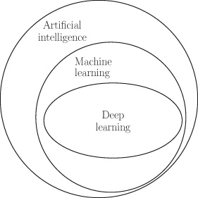
Figure 1.1 The relationship between artificial intelligence, machine learning, and deep learning. Machine learning involves the development and evaluation of algorithms that enable a computer to extract (or learn) functions from a dataset (sets of examples). To understand what machine learning means we need to understand three terms: dataset, algorithm, and function.
In its simplest form, a dataset is a table where each row contains the description of one example from a domain, and each column contains the information for one of the features in a domain. For example, table 1.1 illustrates an example dataset for a loan application domain. This dataset lists the details of four example loan applications. Excluding the ID feature, which is only for ease of reference, each example is described using three features: the applicant’s annual income, their current debt, and their credit solvency.
Table 1.1. A dataset of loan applicants and their known credit solvency ratings
ID Annual Income Current Debt Credit Solvency 1 $150 -$100 100 2 $250 -$300 -50 3 $450 -$250 400 4 $200 -$350 -300 An algorithm is a process (or recipe, or program) that a computer can follow. In the context of machine learning, an algorithm defines a process to analyze a dataset and identify recurring patterns in the data. For example, the algorithm might find a pattern that relates a person’s annual income and current debt to their credit solvency rating. In mathematics, relationships of this type are referred to as functions.
A function is a deterministic mapping from a set of input values to one or more output values. The fact that the mapping is deterministic means that for any specific set of inputs a function will always return the same outputs. For example, addition is a deterministic mapping, and so 2+2 is always equal to 4. As we will discuss later, we can create functions for domains that are more complex than basic arithmetic, we can for example define a function that takes a person’s income and debt as inputs and returns their credit solvency rating as the output value. The concept of a function is very important to deep learning so it is worth repeating the definition for emphasis: a function is simply a mapping from inputs to outputs. In fact, the goal of machine learning is to learn functions from data. A function can be represented in many different ways: it can be as simple as an arithmetic operation (e.g., addition or subtraction are both functions that take inputs and return a single output), a sequence of if-then-else rules, or it can have a much more complex representation.
A function is a deterministic mapping from a set of input values to one or more output values.
One way to represent a function is to use a neural network. Deep learning is the subfield of machine learning that focuses on deep neural network models. In fact, the patterns that deep learning algorithms extract from datasets are functions that are represented as neural networks. Figure 1.2 illustrates the structure of a neural network. The boxes on the left of the figure represent the memory locations where inputs are presented to the network. Each of the circles in this figure is called a neuron and each neuron implements a function: it takes a number of values as input and maps them to an output value. The arrows in the network show how the outputs of each neuron are passed as inputs to other neurons. In this network, information flows from left to right. For example, if this network were trained to predict a person’s credit solvency, based on their income and debt, it would receive the income and debt as inputs on the left of the network and output the credit solvency score through the neuron on the right.
A neural network uses a divide-and-conquer strategy to learn a function: each neuron in the network learns a simple function, and the overall (more complex) function, defined by the network, is created by combining these simpler functions. Chapter 3 will describe how a neural network processes information.
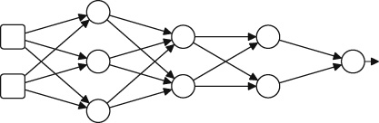
Figure 1.2 Schematic illustration of a neural network. What Is Machine Learning?
A machine learning algorithm is a search process designed to choose the best function, from a set of possible functions, to explain the relationships between features in a dataset. To get an intuitive understanding of what is involved in extracting, or learning, a function from data, examine the following set of sample inputs to an unknown function and the outputs it returns. Given these examples, decide which arithmetic operation (addition, subtraction, multiplication, or division) is the best choice to explain the mapping the unknown function defines between its inputs and output:
Most people would agree that multiplication is the best choice because it provides the best match to the observed relationship, or mapping, from the inputs to the outputs:
In this particular instance, choosing the best function is relatively straightforward, and a human can do it without the aid of a computer. However, as the number of inputs to the unknown function increases (perhaps to hundreds or thousands of inputs), and the variety of potential functions to be considered gets larger, the task becomes much more difficult. It is in these contexts that harnessing the power of machine learning to search for the best function, to match the patterns in the dataset, becomes necessary.
Machine learning involves a two-step process: training and inference. During training, a machine learning algorithm processes a dataset and chooses the function that best matches the patterns in the data. The extracted function will be encoded in a computer program in a particular form (such as if-then-else rules or parameters of a specified equation). The encoded function is known as a model, and the analysis of the data in order to extract the function is often referred to as training the model. Essentially, models are functions encoded as computer programs. However, in machine learning the concepts of function and model are so closely related that the distinction is often skipped over and the terms may even be used interchangeably.
In the context of deep learning, the relationship between functions and models is that the function extracted from a dataset during training is represented as a neural network model, and conversely a neural network model encodes a function as a computer program. The standard process used to train a neural network is to begin training with a neural network where the parameters of the network are randomly initialized (we will explain network parameters later; for now just think of them as values that control how the function the network encodes works). This randomly initialized network will be very inaccurate in terms of its ability to match the relationship between the various input values and target outputs for the examples in the dataset. The training process then proceeds by iterating through the examples in the dataset, and, for each example, presenting the input values to the network and then using the difference between the output returned by the network and the correct output for the example listed in the dataset to update the network’s parameters so that it matches the data more closely. Once the machine learning algorithm has found a function that is sufficiently accurate (in terms of the outputs it generates matching the correct outputs listed in the dataset) for the problem we are trying to solve, the training process is completed, and the final model is returned by the algorithm. This is the point at which the learning in machine learning stops.
Once training has finished, the model is fixed. The second stage in machine learning is inference. This is when the model is applied to new examples—examples for which we do not know the correct output value, and therefore we want the model to generate estimates of this value for us. Most of the work in machine learning is focused on how to train accurate models (i.e., extracting an accurate function from data). This is because the skills and methods required to deploy a trained machine learning model into production, in order to do inference on new examples at scale, are different from those that a typical data scientist will possess. There is a growing recognition within the industry of the distinctive skills needed to deploy artificial intelligence systems at scale, and this is reflected in a growing interest in the field known as DevOps, a term describing the need for collaboration between development and operations teams (the operations team being the team responsible for deploying a developed system into production and ensuring that these systems are stable and scalable). The terms MLOps, for machine learning operations, and AIOps, for artificial intelligence operations, are also used to describe the challenges of deploying a trained model. The questions around model deployment are beyond the scope of this book, so we will instead focus on describing what deep learning is, what it can be used for, how it has evolved, and how we can train accurate deep learning models.
One relevant question here is: why is extracting a function from data useful? The reason is that once a function has been extracted from a dataset it can be applied to unseen data, and the values returned by the function in response to these new inputs can provide insight into the correct decisions for these new problems (i.e., it can be used for inference). Recall that a function is simply a deterministic mapping from inputs to outputs. The simplicity of this definition, however, hides the variety that exists within the set of functions. Consider the following examples:
- • Spam filtering is a function that takes an email as input and returns a value that classifies the email as spam (or not).
- • Face recognition is a function that takes an image as input and returns a labeling of the pixels in the image that demarcates the face in the image.
- • Gene prediction is a function that takes a genomic DNA sequence as input and returns the regions of the DNA that encode a gene.
- • Speech recognition is a function that takes an audio speech signal as input and returns a textual transcription of the speech.
- • Machine translation is a function that takes a sentence in one language as input and returns the translation of that sentence in another language.
It is because the solutions to so many problems across so many domains can be framed as functions that machine learning has become so important in recent years.
Why Is Machine Learning Difficult?
There are a number of factors that make the machine learning task difficult, even with the help of a computer. First, most datasets will include noise3 in the data, so searching for a function that matches the data exactly is not necessarily the best strategy to follow, as it is equivalent to learning the noise. Second, it is often the case that the set of possible functions is larger than the set of examples in the dataset. This means that machine learning is an ill-posed problem: the information given in the problem is not sufficient to find a single best solution; instead multiple possible solutions will match the data. We can use the problem of selecting the arithmetic operation (addition, subtraction, multiplication, or division) that best matches a set of example input-output mappings for an unknown function to illustrate the concept of an ill-posed problem. Here are the example mappings for this function selection problem:
Given these examples, multiplication and division are better matches for the unknown function than addition and subtraction. However, it is not possible to decide whether the unknown function is actually multiplication or division using this sample of data, because both operations are consistent with all the examples provided. Consequently, this is an ill-posed problem: it is not possible to select a single best answer given the information provided in the problem.
One strategy to solve an ill-posed problem is to collect more data (more examples) in the hope that the new examples will help us to discriminate between the correct underlying function and the remaining alternatives. Frequently, however, this strategy is not feasible, either because the extra data is not available or is too expensive to collect. Instead, machine learning algorithms overcome the ill-posed nature of the machine learning task by supplementing the information provided by the data with a set of assumptions about the characteristics of the best function, and use these assumptions to influence the process used by the algorithm that selects the best function (or model). These assumptions are known as the inductive bias of the algorithm because in logic a process that infers a general rule from a set of specific examples is known as inductive reasoning. For example, if all the swans that you have seen in your life are white, you might induce from these examples the general rule that all swans are white. This concept of inductive reasoning relates to machine learning because a machine learning algorithm induces (or extracts) a general rule (a function) from a set of specific examples (the dataset). Consequently, the assumptions that bias a machine learning algorithm are, in effect, biasing an inductive reasoning process, and this is why they are known as the inductive bias of the algorithm.
So, a machine learning algorithm uses two sources of information to select the best function: one is the dataset, and the other (the inductive bias) is the assumptions that bias the algorithm to prefer some functions over others, irrespective of the patterns in the dataset. The inductive bias of a machine learning algorithm can be understood as providing the algorithm with a perspective on a dataset. However, just as in the real world, where there is no single best perspective that works in all situations, there is no single best inductive bias that works well for all datasets. This is why there are so many different machine learning algorithms: each algorithm encodes a different inductive bias. The assumptions encoded in the design of a machine leanring algorithm can vary in strength. The stronger the assumptions the less freedom the algorithm is given in selecting a function that fits the patterns in the dataset. In a sense, the dataset and inductive bias counterbalance each other: machine learning algorithms that have a strong inductive bias pay less attention to the dataset when selecting a function. For example, if a machine learning algorithm is coded to prefer a very simple function, no matter how complex the patterns in the data, then it has a very strong inductive bias.
In chapter 2 we will explain how we can use the equation of a line as a template structure to define a function. The equation of the line is a very simple type of mathematical function. Machine learning algorithms that use the equation of a line as the template structure for the functions they fit to a dataset make the assumption that the model they generate should encode a simple linear mapping from inputs to output. This assumption is an example of an inductive bias. It is, in fact, an example of a strong inductive bias, as no matter how complex (or nonlinear) the patterns in the data are the algorithm will be restricted (or biased) to fit a linear model to it.
One of two things can go wrong if we choose a machine learning algorithm with the wrong bias. First, if the inductive bias of a machine learning algorithm is too strong, then the algorithm will ignore important information in the data and the returned function will not capture the nuances of the true patterns in the data. In other words, the returned function will be too simple for the domain,4 and the outputs it generates will not be accurate. This outcome is known as the function underfitting the data. Alternatively, if the bias is too weak (or permissive), the algorithm is allowed too much freedom to find a function that closely fits the data. In this case, the returned function is likely to be too complex for the domain, and, more problematically, the function is likely to fit to the noise in the sample of the data that was supplied to the algorithm during training. Fitting to the noise in the training data will reduce the function’s ability to generalize to new data (data that is not in the training sample). This outcome is known as overfitting the data. Finding a machine learning algorithm that balances data and inductive bias appropriately for a given domain is the key to learning a function that neither underfits or overfits the data, and that, therefore, generalizes successfully in that domain (i.e., that is accurate at inference, or processing new examples that were not in the training data).
However, in domains that are complex enough to warrant the use of machine learning, it is not possible in advance to know what are the correct assumptions to use to bias the selection of the correct model from the data. Consequently, data scientists must use their intuition (i.e., make informed guesses) and also use trial-and-error experimentation in order to find the best machine learning algorithm to use in a given domain.
Neural networks have a relatively weak inductive bias. As a result, generally, the danger with deep learning is that the neural network model will overfit, rather than underfit, the data. It is because neural networks pay so much attention to the data that they are best suited to contexts where there are very large datasets. The larger the dataset, the more information the data provides, and therefore it becomes more sensible to pay more attention to the data. Indeed, one of the most important factors driving the emergence of deep learning over the last decade has been the emergence of Big Data. The massive datasets that have become available through online social platforms and the proliferation of sensors have combined to provide the data necessary to train neural network models to support new applications in a range of domains. To give a sense of the scale of the big data used in deep learning research, Facebook’s face recognition software, DeepFace, was trained on a dataset of four million facial images belonging to more than four thousand identities (Taigman et al. 2014).
The Key Ingredients of Machine Learning
The above example of deciding which arithmetic operation best explains the relationship between inputs and outputs in a set of data illustrates the three key ingredients in machine learning:
1. Data (a set of historical examples).
2. A set of functions that the algorithm will search through to find the best match with the data.
3. Some measure of fitness that can be used to evaluate how well each candidate function matches the data.All three of these ingredients must be correct if a machine learning project is to succeed; below we describe each of these ingredients in more detail.
We have already introduced the concept of a dataset as a two-dimensional table (or n × m matrix),5 where each row contains the information for one example, and each column contains the information for one of the features in the domain. For example, table 1.2 illustrates how the sample inputs and outputs of the first unknown arithmetic function problem in the chapter can be represented as a dataset. This dataset contains four examples (also known as instances), and each example is represented using two input features and one output (or target) feature. Designing and selecting the features to represent the examples is a very important step in any machine learning project.
As is so often the case in computer science, and machine learning, there is a tradeoff in feature selection. If we choose to include only a minimal number of features in the dataset, then it is likely that a very informative feature will be excluded from the data, and the function returned by the machine learning algorithm will not work well. Conversely, if we choose to include as many features as possible in the domain, then it is likely that irrelevant or redundant features will be included, and this will also likely result in the function not working well. One reason for this is that the more redundant or irrelevant features that are included, the greater the probability for the machine learning algorithm to extract patterns that are based on spurious correlations between these features. In these cases, the algorithm gets confused between the real patterns in the data and the spurious patterns that only appear in the data due to the particular sample of examples that have been included in the dataset.
Finding the correct set of features to include in a dataset involves engaging with experts who understand the domain, using statistical analysis of the distribution of individual features and also the correlations between pairs of features, and a trial-and-error process of building models and checking the performance of the models when particular features are included or excluded. This process of dataset design is a labor-intensive task that often takes up a significant portion of the time and effort expended on a machine learning project. It is, however, a critical task if the project is to succeed. Indeed, identifying which features are informative for a given task is frequently where the real value of machine learning projects emerge.
The second ingredient in a machine learning project is the set of candidate functions that the algorithm will consider as the potential explanation of the patterns in the data. In the unknown arithmetic function scenario previously given, the set of considered functions was explicitly specified and restricted to four: addition, subtraction, multiplication, or division. More generally, the set of functions is implicitly defined through the inductive bias of the machine learning algorithm and the function representation (or model) that is being used. For example, a neural network model is a very flexible function representation.
Table 1.2. A simple tabular dataset
Input 1 Input 2 Target 5 5 25 2 6 12 4 4 16 2 2 04 The third and final ingredient to machine learning is the measure of fitness. The measure of fitness is a function that takes the outputs from a candidate function, generated when the machine learning algorithm applies the candidate function to the data, and compares these outputs with the data, in some way. The result of this comparison is a value that describes the fitness of the candidate function relative to the data. A fitness function that would work for our unknown arithmetic function scenario is to count in how many of the examples a candidate function returns a value that exactly matches the target specified in the data. Multiplication would score four out of four on this fitness measure, addition would score one out of four, and division and subtraction would both score zero out of four. There are a large variety of fitness functions that can be used in machine learning, and the selection of the correct fitness function is crucial to the success of a machine learning project. The design of new fitness functions is a rich area of research in machine learning. Varying how the dataset is represented, and how the candidate functions and the fitness function are defined, results in three different categories of machine learning: supervised, unsupervised, and reinforcement learning.
Supervised, Unsupervised, and Reinforcement Learning
Supervised machine learning is the most common type of machine learning. In supervised machine learning, each example in the dataset is labeled with the expected output (or target) value. For example, if we were using the dataset in table 1.1 to learn a function that maps from the inputs of annual income and debt to a credit solvency score, the credit solvency feature in the dataset would be the target feature. In order to use supervised machine learning, our dataset must list the value of the target feature for every example in the dataset. These target feature values can sometimes be very difficult, and expensive, to collect. In some cases, we must pay human experts to label each example in a dataset with the correct target value. However, the benefit of having these target values in the dataset is that the machine learning algorithm can use these values to help the learning process. It does this by comparing the outputs a function produces with the target outputs specified in the dataset, and using the difference (or error) to evaluate the fitness of the candidate function, and use the fitness evaluation to guide the search for the best function. It is because of this feedback from the target labels in the dataset to the algorithm that this type of machine learning is considered supervised. This is the type of machine learning that was demonstrated by the example of choosing between different arithmetic functions to explain the behavior of an unknown function.
Unsupervised machine learning is generally used for clustering data. For example, this type of data analysis is useful for customer segmentation, where a company wishes to segment its customer base into coherent groups so that it can target marketing campaigns and/or product designs to each group. In unsupervised machine learning, there are no target values in the dataset. Consequently, the algorithm cannot directly evaluate the fitness of a candidate function against the target values in the dataset. Instead, the machine learning algorithm tries to identify functions that map similar examples into clusters, such that the examples in a cluster are more similar to the other examples in the same cluster than they are to examples in other clusters. Note that the clusters are not prespecified, or at most they are initially very underspecified. For example, the data scientist might provide the algorithm with a target number of clusters, based on some intuition about the domain, without providing explicit information on relative sizes of the clusters or regarding the characteristics of examples that belong in each cluster. Unsupervised machine learning algorithms often begin by guessing an initial clustering of the examples and then iteratively adjusting the clusters (by dropping instances from one cluster and adding them to another) so as to improve the fitness of the cluster set. The fitness functions used in unsupervised machine learning generally reward candidate functions that result in higher similarity within individual clusters and, also, high diversity between clusters.
Reinforcement learning is most relevant for online control tasks, such as robot control and game playing. In these scenarios, an agent needs to learn a policy for how it should act in an environment in order to be rewarded. In reinforcement learning, the goal of the agent is to learn a mapping from its current observation of the environment and its own internal state (its memory) to what action it should take: for instance, should the robot move forward or backward or should the computer program move the pawn or take the queen. The output of this policy (function) is the action that the agent should take next, given the current context. In these types of scenarios, it is difficult to create historic datasets, and so reinforcement learning is often carried out in situ: an agent is released into an environment where it experiments with different policies (starting with a potentially random policy) and over time updates its policy in response to the rewards it receives from the environment. If an action results in a positive reward, the mapping from the relevant observations and state to that action is reinforced in the policy, whereas if an action results in a negative reward, the mapping is weakened. Unlike in supervised and unsupervised machine learning, in reinforcement learning, the fact that learning is done in situ means that the training and inference stages are interleaved and ongoing. The agent infers what action it should do next and uses the feedback from the environment to learn how to update its policy. A distinctive aspect of reinforcement learning is that the target output of the learned function (the agent’s actions) is decoupled from the reward mechanism. The reward may be dependent on multiple actions and there may be no reward feedback, either positive or negative, available directly after an action has been performed. For example, in a chess scenario, the reward may be +1 if the agent wins the game and -1 if the agent loses. However, this reward feedback will not be available until the last move of the game has been completed. So, one of the challenges in reinforcement learning is designing training mechanisms that can distribute the reward appropriately back through a sequence of actions so that the policy can be updated appropriately. Google’s DeepMind Technologies generated a lot of interest by demonstrating how reinforcement learning could be used to train a deep learning model to learn control policies for seven different Atari computer games (Mnih et al. 2013). The input to the system was the raw pixel values from the screen, and the control policies specified what joystick action the agent should take at each point in the game. Computer game environments are particularly suited to reinforcement learning as the agent can be allowed to play many thousands of games against the computer game system in order to learn a successful policy, without incurring the cost of creating and labeling a large dataset of example situations with correct joystick actions. The DeepMind system got so good at the games that it outperformed all previous computer systems on six of the seven games, and outperformed human experts on three of the games.
Deep learning can be applied to all three machine learning scenarios: supervised, unsupervised, and reinforcement. Supervised machine learning is, however, the most common type of machine learning. Consequently, the majority of this book will focus on deep learning in a supervised learning context. However, most of the deep learning concerns and principles introduced in the supervised learning context also apply to unsupervised and reinforcement learning.
Why Is Deep Learning So Successful?
In any data-driven process the primary determinant of success is knowing what to measure and how to measure it. This is why the processes of feature selection and feature design are so important to machine learning. As discussed above, these tasks can require domain expertise, statistical analysis of the data, and iterations of experiments building models with different feature sets. Consequently, dataset design and preparation can consume a significant portion of time and resources expended in the project, in some cases approaching up to 80% of the total budget of a project (Kelleher and Tierney 2018). Feature design is one task in which deep learning can have a significant advantage over traditional machine learning. In traditional machine learning, the design of features often requires a large amount of human effort. Deep learning takes a different approach to feature design, by attempting to automatically learn the features that are most useful for the task from the raw data.
In any data-driven process the primary determinant of success is knowing what to measure and how to measure it.
To give an example of feature design, a person’s body mass index (BMI) is the ratio of a person’s weight (in kilograms) divided by their height (in meters squared). In a medical setting, BMI is used to categorize people as underweight, normal, overweight, or obese. Categorizing people in this way can be useful in predicting the likelihood of a person developing a weight-related medical condition, such as diabetes. BMI is used for this categorization because it enables doctors to categorize people in a manner that is relevant to these weight-related medical conditions. Generally, as people get taller they also get heavier. However, most weight-related medical conditions (such as diabetes) are not affected by a person’s height but rather the amount they are overweight compared to other people of a similar stature. BMI is a useful feature to use for the medical categorization of a person’s weight because it takes the effect of height on weight into account. BMI is an example of a feature that is derived (or calculated) from raw features; in this case the raw features are weight and height. BMI is also an example of how a derived feature can be more useful in making a decision than the raw features that it is derived from. BMI is a hand-designed feature: Adolphe Quetelet designed it in the eighteenth century.
As mentioned above, during a machine learning project a lot of time and effort is spent on identifying, or designing, (derived) features that are useful for the task the project is trying to solve. The advantage of deep learning is that it can learn useful derived features from data automatically (we will discuss how it does this in later chapters). Indeed, given large enough datasets, deep learning has proven to be so effective in learning features that deep learning models are now more accurate than many of the other machine learning models that use hand-engineered features. This is also why deep learning is so effective in domains where examples are described with very large numbers of features. Technically datasets that contain large numbers of features are called high-dimensional. For example, a dataset of photos with a feature for each pixel in a photo would be high-dimensional. In complex high-dimensional domains, it is extremely difficult to hand-engineer features: consider the challenges of hand-engineering features for face recognition or machine translation. So, in these complex domains, adopting a strategy whereby the features are automatically learned from a large dataset makes sense. Related to this ability to automatically learn useful features, deep learning also has the ability to learn complex nonlinear mappings between inputs and outputs; we will explain the concept of a nonlinear mapping in chapter 3, and in chapter 6 we will explain how these mappings are learned from data.
Summary and the Road Ahead
This chapter has focused on positioning deep learning within the broader field of machine learning. Consequently, much of this chapter has been devoted to introducing machine learning. In particular, the concept of a function as a deterministic mapping from inputs to outputs was introduced, and the goal of machine learning was explained as finding a function that matches the mappings from input features to the output features that are observed in the examples in the dataset.
Within this machine learning context, deep learning was introduced as the subfield of machine learning that focuses on the design and evaluation of training algorithms and model architectures for modern neural networks. One of the distinctive aspects of deep learning within machine learning is the approach it takes to feature design. In most machine learning projects, feature design is a human-intensive task that can require deep domain expertise and consume a lot of time and project budget. Deep learning models, on the other hand, have the ability to learn useful features from low-level raw data, and complex nonlinear mappings from inputs to outputs. This ability is dependent on the availability of large datasets; however, when such datasets are available, deep learning can frequently outperform other machine learning approaches. Furthermore, this ability to learn useful features from large datasets is why deep learning can often generate highly accurate models for complex domains, be it in machine translation, speech processing, or image or video processing. In a sense, deep learning has unlocked the potential of big data. The most noticeable impact of this development has been the integration of deep learning models into consumer devices. However, the fact that deep learning can be used to analyze massive datasets also has implications for our individual privacy and civil liberty (Kelleher and Tierney 2018). This is why understanding what deep learning is, how it works, and what it can and can’t be used for, is so important. The road ahead is as follows:
• Chapter 2 introduces some of the foundational concepts of deep learning, including what a model is, how the parameters of a model can be set using data, and how we can create complex models by combining simple models.
• Chapter 3 explains what neural networks are, how they work, and what we mean by a deep neural network.
• Chapter 4 presents a history of deep learning. This history focuses on the major conceptual and technical breakthroughs that have contributed to the development of the field of machine learning. In particular, it provides a context and explanation for why deep learning has seen such rapid development in recent years.
• Chapter 5 describes the current state of the field, by introducing the two deep neural architectures that are the most popular today: convolutional neural networks and recurrent neural networks. Convolutional neural networks are ideally suited to processing image and video data. Recurrent neural networks are ideally suited to processing sequential data such as speech, text, or time-series data. Understanding the differences and commonalities across these two architectures will give you an awareness of how a deep neural network can be tailored to the characteristics of a specific type of data, and also an appreciation of the breadth of the design space of possible network architectures.
• Chapter 6 explains how deep neural networks models are trained, using the gradient descent and backpropagation algorithms. Understanding these two algorithms will give you a real insight into the state of artificial intelligence. For example, it will help you to understand why, given enough data, it is currently possible to train a computer to do a specific task within a well-defined domain at a level beyond human capabilities, but also why a more general form of intelligence is still an open research challenge for artificial intelligence.
• Chapter 7 looks to the future in the field of deep learning. It reviews the major trends driving the development of deep learning at present, and how they are likely to contribute to the development of the field in the coming years. The chapter also discusses some of the challenges the field faces, in particular the challenge of understanding and interpreting how a deep neural network works.2 Conceptual Foundations
This chapter introduces some of the foundational concepts that underpin deep learning. The basis of this chapter is to decouple the initial presentation of these concepts from the technical terminology used in deep learning, which is introduced in subsequent chapters.
A deep learning network is a mathematical model that is (loosely) inspired by the structure of the brain. Consequently, in order to understand deep learning it is helpful to have an intuitive understanding of what a mathematical model is, how the parameters of a model can be set, how we can combine (or compose) models, and how we can use geometry to understand how a model processes information.
What Is a Mathematical Model?
In its simplest form, a mathematical model is an equation that describes how one or more input variables are related to an output variable. In this form a mathematical model is the same as a function: a mapping from inputs to outputs.
In any discussion relating to models, it is important to remember the statement by George Box that all models are wrong but some are useful! For a model to be useful it must have a correspondence with the real world. This correspondence is most obvious in terms of the meaning that can be associated with a variable. For example, in isolation a value such as 78,000 has no meaning because it has no correspondence with concepts in the real world. But yearly income=$78,000 tells us how the number describes an aspect of the real world. Once the variables in a model have a meaning, we can understand the model as describing a process through which different aspects of the world interact and cause new events. The new events are then described by the outputs of the model.
A very simple template for a model is the equation of a line:

In this equation
is the output variable,
is the input variable, and
and
are two parameters of the model that we can set to adjust the relationship the model defines between the input and the output.
Imagine we have a hypothesis that yearly income affects a person’s happiness and we wish to describe the relationship between these two variables.1 Using the equation of a line, we could define a model to describe this relationship as follows:

This model has a meaning because the variables in the model (as distinct from the parameters of the model) have a correspondence with concepts from the real world. To complete our model, we have to set the values of the model’s parameters:
and
. Figure 2.1 illustrates how varying the values of each of these parameters changes the relationship defined by the model between income and happiness.
One important thing to notice in this figure is that no matter what values we set the model parameters to, the relationship defined by the model between the input and the output variable can be plotted as a line. This is not surprising because we used the equation of a line as the template to define our model, and this is why mathematical models that are based on the equation of a line are known as linear models. The other important thing to notice in the figure is how changing the parameters of the model changes the relationship between income and happiness.
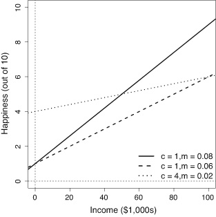
Figure 2.1 Three different linear models of how income affects happiness. The solid steep line, with parameters
, is a model of the world in which people with zero income have a happiness level of 1, and increases in income have a significant effect on people’s happiness. The dashed line, with parameters
, is a model in which people with zero income have a happiness level of 1 and increased income increases happiness, but at the slower rate compared to the world modeled by the solid line. Finally, the dotted line, parameters
, is a model of the world where no one is particularly unhappy—even people with zero income have a happiness of 4 out of 10—and although increases in income do affect happiness, the effect is moderate. This third model assumes that income has a relatively weak effect on happiness.
More generally, the differences between the three models in figure 2.1 show how making changes to the parameters of a linear model changes the model. Changing
causes the line to move up and done. This is most clearly seen if we focus on the y-axis: notice that the line defined by a model always crosses (or intercepts) the y-axis at the value that
is set to. This is why the
parameter in a linear model is known as the intercept. The intercept can be understood as specifying the value of the output variable when the input variable is zero. Changing the
parameter changes the angle (or slope) of the line. The slope parameter controls how quickly changes in income effect changes in happiness. In a sense, the slope value is a measure of how important income is to happiness. If income is very important (i.e., if small changes in income result in big changes in happiness), then the slope parameter of our model should be set to a large value. Another way of understanding this is to think of a slope parameter of a linear model as describing the importance, or weight, of the input variable in determining the value of the output.
Linear Models with Multiple Inputs
The equation of a line can be used as a template for mathematical models that have more than one input variable. For example, imagine yourself in a scenario where you have been hired by a financial institution to act as a loan officer and your job involves deciding whether or not a loan application should be granted. From interviewing domain experts you come up with a hypothesis that a useful way to model a person’s credit solvency is to consider both their yearly income and their current debts. If we assume that there is a linear relationship between these two input variables and a person’s credit solvency, then the appropriate mathematical model, written out in English would be:
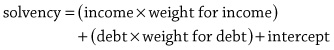
Notice that in this model the
m
parameter has been replaced by a separate weight for each input variable, with each weight representing the importance of its associated input in determining the output. In mathematical notation this model would be written as:
where
represents the credit solvency output,
represents the income variable,
represents the debt variable, and
represents the intercept. Using the idea of adding a new weight for each new input to the model allows us to scale the equation of a line to as many inputs as we like. All the models defined in this way are still linear within the dimensions defined by the number of inputs and the output. What this means is that a linear model with two inputs and one output defines a flat plane rather than a line because that is what a two-dimensional line that has been extruded to three dimensions looks like.It can become tedious to write out a mathematical model that has a lot of inputs, so mathematicians like to write things in as compact a form as possible. With this in mind, the above equation is sometimes written in the short form:
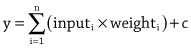
This notation tells us that to calculate the output variable
y
we must first go through all
inputs and multiple each input by its corresponding weight, then we should sum together the results of these
multiplications, and finally we add the
intercept parameter to the result of the summation. The
symbol tells us that we use addition to combine the results of the multiplications, and the index
tells us that we multiply each input by the weight with the same index. We can make our notation even more compact by treating the intercept as a weight. One way to do this is to assume an
that is always equal to 1 and to treat the intercept as the weight on this input, that is,
. Doing this allows us to write out the model as follows: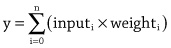
Notice that the index now starts at 0, rather than 1, because we are now assuming an extra input,
input0=1
, and we have relabeled the intercept
weight0.Although we can write down a linear model in a number of different ways, the core of a linear model is that the output is calculated as the sum of the n input values multiplied by their corresponding weights. Consequently, this type of model defines a calculation known as a weighted sum, because we weight each input and sum the results. Although a weighted sum is easy to calculate, it turns out to be very useful in many situations, and it is the basic calculation used in every neuron in a neural network.
Setting the Parameters of a Linear Model
Let us return to our working scenario where we wish to create a model that enables us to calculate the credit solvency of individuals who have applied for a financial loan. For simplicity in presentation we will ignore the intercept parameter in this discussion as it is treated the same as the other parameters (i.e., the weights on the inputs). So, dropping the intercept parameter, we have the following linear model (or weighted sum) of the relationship between a person’s income and debt to their credit solvency:
The multiplication of inputs by weights, followed by a summation, is known as a weighted sum.
In order to complete our model, we need to specify the parameters of the model; that is, we need to specify the value of the weight for each input. One way to do this would be to use our domain expertise to come up with values for each of the parameters.
For example, if we assume that an increase in a person’s income has a bigger impact on their credit solvency than a similar increase in their debt, we should set the weighting for income to be larger than that of the debt. The following model encodes this assumption; in particular this model specifies that income is three times as important as debt in determining a person’s credit solvency:
The drawback with using domain knowledge to set the parameters of a model is that experts often disagree. For example, you may think that weighting income as three times as important as debt is not realistic; in that case the model can be adjusted by, for example, setting both income and debt to have an equal weighting, which would be equivalent to assuming that income and debt are equally important in determining credit solvency. One way to avoid arguments between experts is to use data to set the parameters. This is where machine learning helps. The learning done by machine learning is finding the parameters (or weights) of a model using a dataset.
Learning Model Parameters from Data
Later in the book we will describe the standard algorithm used to learn the weights for a linear model, known as the gradient descent algorithm. However, we can give a brief preview of the algorithm here. We start with a dataset containing a set of examples for which we have both the input values (income and debt) and the output value (credit solvency). Table 2.1 illustrates such a dataset from our credit solvency scenario.2
The learning done by machine learning is finding the parameters (or weights) of a model using a dataset.
We then begin the process of learning the weights by guessing initial values for each weight. It is very likely that this initial, guessed, model will be a very bad model. This is not a problem, however, because we will use the dataset to iteratively update the weights so that the model gets better and better, in terms of how well it matches the data. For the purpose of the example, we will use the model described above as our initial (guessed) model:
Table 2.1. A dataset of loan applications and known credit solvency rating of the applicant
ID Annual income Current debt Credit solvency 1 $150 -$100 100 2 $250 -$300 -50 3 $450 -$250 400 4 $200 -$350 -300 The general process for improving the weights of the model is to select an example from the dataset and feed the input values from the example into the model. This allows us to calculate an estimate of the output value for the example. Once we have this estimated output, we can calculate the error of the model on the example by subtracting the estimated output from the correct output for the example listed in the dataset. Using the error of the model on the example, we can improve how well the model fits the data by updating the weights in the model using the following strategy, or learning rule:
• If the error is 0, then we should not change the weights of the model.
• If the error is positive, then the output of the model was too low, so we should increase the output of the model for this example by increasing the weights for all the inputs that had positive values for the example and decreasing the weights for all the inputs that had negative values for the example.
• If the error is negative, then the output of the model was too high, so we should decrease the output of the model for this example by decreasing the weights for all the inputs that had positive values for the example and increasing the weights for all the inputs that had negative values for the example.To illustrate the weight update process we will use example 1 from table 2.1 (income = 150, debt = -100, and solvency = 100) to test the accuracy of our guessed model and update the weights according to the resulting error.
When the input values for the example are passed into the model, the credit solvency estimate returned by the model is 350. This is larger than the credit solvency listed for this example in the dataset, which is 100. As a result, the error of the model is negative (100 – 350 = –250); therefore, following the learning rule described above, we should decrease the output of the model for this example by decreasing the weights for positive inputs and increasing the weights for negative inputs. For this example, the income input had a positive value and the debt input had a negative value. If we decrease the weight for income by 1 and increase the weight for debt by 1, we end up with the following model:
We can test if this weight update has improved the model by checking if the new model generates a better estimate for the example than the old model. The following illustrates pushing the same example through the new model:
This time the credit solvency estimate generated by the model matches the value in the dataset, showing that the updated model fits the data more closely than the original model. In fact, this new model generates the correct output for all the examples in the dataset.
In this example, we only needed to update the weights once in order to find a set of weights that made the behavior of the model consistent with all the examples in the dataset. Typically, however, it takes many iterations of presenting examples and updating weights to get a good model. Also, in this example, we have, for the sake of simplicity, assumed that the weights are updated by either adding or subtracting 1 from them. Generally, in machine learning, the calculation of how much to update each weight by is more complicated than this. However, these differences aside, the general process outlined here for updating the weights (or parameters) of a model in order to fit the model to a dataset is the learning process at the core of deep learning.
Combining Models
We now understand how we can specify a linear model to estimate an applicant’s credit solvency, and how we can modify the parameters of the model in order to fit the model to a dataset. However, as a loan officer our job is not simply to calculate an applicant’s credit solvency; we have to decide whether to grant the loan application or not. In other words, we need a rule that will take a credit solvency score as input and return a decision on the loan application. For example, we might use the decision rule that a person with a credit solvency above 200 will be granted a loan. This decision rule is also a model: it maps an input variable, in this case credit solvency, to an output variable, loan decision.
Using this decision rule we can adjudicate on a loan application by first using the model of credit solvency to convert a loan applicant’s profile (described in terms of the annual income and debt) into a credit solvency score, and then passing the resulting credit solvency score through our decision rule model to generate the loan decision. We can write this process out in a pseudomathematical shorthand as follows:
Using this notation, the entire decision process for adjudicating the loan application for example 1 from table 2.1 is:
We are now in a position where we can use a model (composed of two simpler models, a decision rule and a weighted sum) to describe how a loan decision is made. What is more, if we use data from previous loan applications to set the parameters (i.e., the weights) of the model, our model will correspond to how we have processed previous loan applications. This is useful because we can use this model to process new applications in a way that is consistent with previous decisions. If a new loan application is submitted, we simply use our model to process the application and generate a decision. It is this ability to apply a mathematical model to new examples that makes mathematical modeling so useful.
When we use the output of one model as the input to another model, we are creating a third model by combining two models. This strategy of building a complex model by combining smaller simpler models is at the core of deep learning networks. As we will see, a neural network is composed of a large number of small units called neurons. Each of these neurons is a simple model in its own right that maps from a set of inputs to an output. The overall model implemented by the network is created by feeding the outputs from one group of neurons as inputs into a second group of neurons and then feeding the outputs of the second group of neurons as inputs to a third group of neurons, as so on, until the final output of the model is generated. The core idea is that feeding the outputs of some neuron as inputs to other neurons enables these subsequent neurons to learn to solve a different part of the overall problem the network is trying to solve by building on the partial solutions implemented by the earlier neurons—in a similar way to the way the decision rule generates the final adjudication for a loan application by building on the calculation of the credit solvency model. We will return to this topic of model composition in subsequent chapters.
Input Spaces, Weight Spaces, and Activation Spaces
Although mathematical models can be written out as equations, it is often useful to understand the geometric meaning of a model. For example, the plots in figure 2.1 helped us understand how changes in the parameters of a linear model changed the relationship between the variables that the model defined. There are a number of geometric spaces that it is useful to distinguish between, and understand, when we are discussing neural networks. These are the input space, the weight space, and the activation space of a neuron. We can use the decision model for loan applications that we defined in the previous section to explain these three different types of spaces.
We will begin by describing the concept of an input space. Our loan decision model took two inputs: the annual income and current debt of the applicant. Table 2.1 listed these input values for four example loan applications. We can plot the input space of this model by treating each of the input variables as the axis of a coordinate system. This coordinate space is referred to as the input space because each point in this space defines a possible combination of input values to the model. For example, the plot at the top-left of figure 2.2 shows the position of each of the four example loan applications within the models input space.
The weight space for a model describes the universe of possible weight combinations that a model might use. We can plot the weight space for a model by defining a coordinate system with one axis per weight in the model. The loan decision model has only two weights, one weight for the annual income input, and one weight for the current debt input. Consequently, the weight space for this model has two dimensions. The plot at the top-right of figure 2.2 illustrates a portion of the weight space for this model. The location of the weight combination used by the model
is highlighted in this figure. Each point within this coordinate system describes a possible set of weights for the model, and therefore corresponds to a different weighted sum function within the model. Consequently, moving from one location to another within this weight space is equivalent to changing the model because it changes the mapping from inputs to output that the model defines.

Figure 2.2 There are four different coordinate spaces related to the processing of the loan decision model: top-left plots the input space; top-right plots the weight space; bottom-left plots the activation (or decision) space; and bottom-right plots the input space with the decision boundary plotted. A linear model maps a set of input values to a point in a new space by applying a weighted sum calculation to the inputs: multiply each input by a weight, and sum the results of the multiplication. In our loan decision model it is in this space that we apply our decision rule. Thus, we could call this space the decision space, but, for reasons that will become clear when we describe the structure of a neuron in the next chapter, we call this space the activation space. The axes of a model’s activation space correspond to the weighted inputs to the model. Consequently, each point in the activation space defines a set of weighted inputs. Applying a decision rule, such as our rule that a person with a credit solvency above 200 will be granted a loan, to each point in this activation space, and recording the result of the decision for each point, enables us to plot the decision boundary of the model in this space. The decision boundary divides those points in the activation space that exceed the threshold, from those points in the space below the threshold. The plot in the bottom-left of figure 2.2 illustrates the activation space for our loan decision model. The positions of the four example loan applications listed in table 2.1 when they are projected into this activation space are shown. The diagonal black line in this figure shows the decision boundary. Using this threshold, loan application number three is granted and the other loan applications are rejected. We can, if we wish, project the decision boundary back into the original input space by recording for each location in the input space which side of the decision boundary in the activation space it is mapped to by the weighted sum function. The plot at the bottom-right of figure 2.2 shows the decision boundary in the original input space (note the change in the values on the axes) and was generated using this process. We will return to the concepts of weight spaces and decision boundaries in next chapter when we describe how adjusting the parameters of a neuron changes the set of input combinations that cause the neuron to output a high activation.
Summary
The main idea presented in this chapter is that a linear mathematical model, be it expressed as an equation or plotted as a line, describes a relationship between a set of inputs and an output. Be aware that not all mathematical models are linear models, and we will come across nonlinear models in this book. However, the fundamental calculation of a weighted sum of inputs does define a linear model. Another big idea introduced in this chapter is that a linear model (a weighted sum) has a set of parameters, that is, the weights used in the weighted sum. By changing these parameters we can change the relationship the model describes between the inputs and the output. If we wish we could set these weights by hand using our domain expertise; however, we can also use machine learning to set the weights of the model so that the behavior of the model fits the patterns found in a dataset. The last big idea introduced in this chapter was that we can build complex models by combining simpler models. This is done by using the output from one (or more) models as input(s) to another model. We used this technique to define our composite model to make loan decisions. As we will see in the next chapter, the structure of a neuron in a neural network is very similar to the structure of this loan decision model. Just like this model, a neuron calculates a weighted sum of its inputs and then feeds the result of this calculation into a second model that decides whether the neuron activates or not.
The focus of this chapter has been to introduce some foundational concepts before we introduce the terminology of machine learning and deep learning. To give a quick overview of how the concepts introduced in this chapter map over to machine learning terminology, our loan decision model is equivalent to a two-input neuron that uses a threshold activation function. The two financial indicators (annual income and current debt) are analogous to the inputs the neuron receives. The terms input vector or feature vector are sometimes used to refer to the set of indicators describing a single example; in this context an example is a single loan applicant, described in terms of two features: annual income and current debt. Also, just like the loan decision model, a neuron associates a weight with each input. And, again, just like the loan decision model, a neuron multiplies each input by its associated weight and sums the results of these multiplications in order to calculate an overall score for the inputs. Finally, similar to the way we applied a threshold to the credit solvency score to convert it into a decision of whether to grant or reject the loan application, a neuron applies a function (known as an activation function) to convert the overall score of the inputs. In the earliest types of neurons, these activation functions were actually threshold functions that worked in exactly the same way as the score threshold used in this credit scoring example. In more recent neural networks, different types of activation functions (for example, the logistic, tanh, or ReLU functions) are used. We will introduce these activation functions in the next chapter.
3 Neural Networks: The Building Blocks of Deep Learning
The term deep learning describes a family of neural network models that have multiple layers of simple information processing programs, known as neurons, in the network. The focus of this chapter is to provide a clear and comprehensive introduction to how these neurons work and are interconnected in artificial neural networks. In later chapters, we will explain how neural networks are trained using data.
A neural network is a computational model that is inspired by the structure of the human brain. The human brain is composed of a massive number of nerve cells, called neurons. In fact, some estimates put the number of neurons in the human brain at one hundred billion (Herculano-Houzel 2009). Neurons have a simple three-part structure consisting of: a cell body, a set of fibers called dendrites, and a single long fiber called an axon. Figure 3.1 illustrates the structure of a neuron and how it connects to other neurons in the brain. The dendrites and the axon stem from the cell body, and the dendrites of one neuron are connected to the axons of other neurons. The dendrites act as input channels to the neuron and receive signals sent from other neurons along their axons. The axon acts as the output channel of a neuron, and so other neurons, whose dendrites are connected to the axon, receive the signals sent along the axon as inputs.
Neurons work in a very simple manner. If the incoming stimuli are strong enough, the neuron transmits an electrical pulse, called an action potential, along its axon to the other neurons that are connected to it. So, a neuron acts as an all-or-none switch, that takes in a set of inputs and either outputs an action potential or no output.
This explanation of the human brain is a significant simplification of the biological reality, but it does capture the main points necessary to understand the analogy between the structure of the human brain and computational models called neural networks. These points of analogy are: (1) the brain is composed of a large number of interconnected and simple units called neurons; (2) the functioning of the brain can be understood as processing information, encoded as high or low electrical signals, or activation potentials, that spread across the network of neurons; and (3) each neuron receives a set of stimuli from its neighbors and maps these inputs to either a high- or low-value output. All computational models of neural networks have these characteristics.
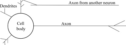
Figure 3.1 The structure of a neuron in the brain. Artificial Neural Networks
An artificial neural network consists of a network of simple information processing units, called neurons. The power of neural networks to model complex relationships is not the result of complex mathematical models, but rather emerges from the interactions between a large set of simple neurons.
Figure 3.2 illustrates the structure of a neural network. It is standard to think of the neurons in a neural network as organized into layers. The depicted network has five layers: one input layer, three hidden layers, and one output layer. A hidden layer is just a layer that is neither the input nor the output layer. Deep learning networks are neural networks that have many hidden layers of neurons. The minimum number of hidden layers necessary to be considered deep is two. However, most deep learning networks have many more than two hidden layers. The important point is that the depth of a network is measured in terms of the number of hidden layers, plus the output layer.
Deep learning networks are neural networks that have many hidden layers of neurons.
In figure 3.2, the squares in the input layer represent locations in memory that are used to present inputs to the network. These locations can be thought of as sensing neurons. There is no processing of information in these sensing neurons; the output of each of these neurons is simply the value of the data stored at the memory location. The circles in the figure represent the information processing neurons in the network. Each of these neurons takes a set of numeric values as input and maps them to a single output value. Each input to a processing neuron is either the output of a sensing neuron or the output of another processing neuron.
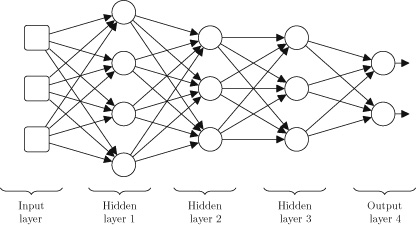
Figure 3.2 Topological illustration of a simple neural network. The arrows in figure 3.2 illustrate how information flows through the network from the output of one neuron to the input of another neuron. Each connection in a network connects two neurons and each connection is directed, which means that information carried along a connection only flows in one direction. Each of the connections in a network has a weight associated with it. A connection weight is simply a number, but these weights are very important. The weight of a connection affects how a neuron processes the information it receives along the connection, and, in fact, training an artificial neural network, essentially, involves searching for the best (or optimal) set of weights.
How an Artificial Neuron Processes Information
The processing of information within a neuron, that is, the mapping from inputs to an output, is very similar to the loan decision model that we developed in chapter 2. Recall that the loan decision model first calculated a weighted sum over the input features (income and debt). The weights used in the weighted sum were adjusted using a dataset so that the results of the weighted sum calculation, given an loan applicant’s income and debt as inputs, was an accurate estimate of the applicant’s credit solvency score. The second stage of processing in the loan decision model involved passing the result of the weighted sum calculation (the estimated credit solvency score) through a decision rule. This decision rule was a function that mapped a credit solvency score to a decision on whether a loan application was granted or rejected.
A neuron also implements a two-stage process to map inputs to an output. The first stage of processing involves the calculation of a weighted sum of the inputs to the neuron. Then the result of the weighted sum calculation is passed through a second function that maps the results of the weighted sum score to the neuron’s final output value. When we are designing a neuron, we can used many different types of functions for this second stage or processing; it may be as simple as the decision rule we used for our loan decision model, or it may be more complex. Typically the output value of a neuron is known as its activation value, so this second function, which maps from the result of the weighted sum to the activation value of the neuron, is known as an activation function.
Figure 3.3 illustrates how these stages of processing are reflected in the structure of an artificial neuron. In figure 3.3, the Σ symbol represents the calculation of the weighted sum, and the φ symbol represents the activation function processing the weighted sum and generating the output from the neuron.
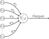
Figure 3.3 The structure of an artificial neuron. The neuron in figure 3.3 receives n inputs
on n different input connections, and each connection has an associated weight
. The weighted sum calculation involves the multiplication of inputs by weights and the summation of the resulting values. Mathematically this calculation is written as:

This calculation can also be written in a more compact mathematical form as:

For example, assuming a neuron received the inputs
and had the following weights
, the weighted sum calculation would be:
z=(3X-3)+(9×1)
=0The second stage of processing within a neuron is to pass the result of the weighted sum, the
value, through an activation function. Figure 3.4 plots the shape of a number of possible activation functions, as the input to each function,
ranges across an interval, either [-1, …, +1] or [-10, …, +10] depending on which interval best illustrates the shape of the function. Figure 3.4 (top) plots a threshold activation function. The decision rule we used in the loan decision model was an example of a threshold function; the threshold used in that decision rule was whether the credit solvency score was above 200. Threshold activations were common in early neural network research. Figure 3.4 (middle) plots the logistic and tanh activation functions. The units employing these activation functions were popular in multilayer networks until quite recently. Figure 3.4 (bottom) plots the rectifier (or hinge, or positive linear) activation function. This activation function is very popular in modern deep learning networks; in 2011 the rectifier activation function was shown to enable better training in deep networks (Glorot et al. 2011). In fact, as will be discussed in chapter 4, during the review of the history of deep learning, one of the trends in neural network research has been a shift from threshold activation to logistic and tanh activations, and then onto rectifier activation functions.
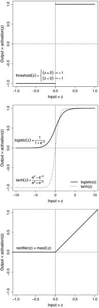
Figure 3.4 Top: threshold function; middle: logistic and tanh functions; bottom: rectified linear function. Returning to the example, the result of the weighted summation step was
. Figure 3.4 (middle plot, solid line) plots the logistic function. Assuming that the neuron is using a logistic activation function, this plot shows how the result of the summation will be mapped to an output activation:
. The calculation of the output activation of this neuron can be summarized as:
Notice that the processing of information in this neuron is nearly identical to the processing of information in the loan decision model we developed in the last chapter. The major difference is that we have replaced the decision threshold rule that mapped the weighted sum score to an accepted or rejected output with a logistic function that maps the weighted sum score to a value between 0 and 1. Depending on the location of this neuron in the network, the output activation of the neuron, in this instance
, will either be passed as input to one or more neurons in the next layer in the network, or will be part of the overall output of the network. If a neuron is at the output layer, the interpretation of what its output value means would be dependent on the task that the neuron is designed to model. If a neuron is in one of the hidden layers of the network, then it may not be possible to put a meaningful interpretation on the output of the neuron apart from the general interpretation that it represents some sort of derived feature (similar to the BMI feature we discussed in chapter 1) that the network has found useful in generating its outputs. We will return to the challenge of interpreting the meaning of activations within a neural network in chapter 7.
The key point to remember from this section is that a neuron, the fundamental building block of neural networks and deep learning, is defined by a simple two-step sequence of operations: calculating a weighted sum and then passing the result through an activation function.
Figure 3.4 illustrates that neither the tanh nor the logistic function is a linear function. In fact, the plots of both of these functions have a distinctive s-shaped (rather than linear) profile. Not all activation functions have an s-shape (for example, the threshold and rectifier are not s-shaped), but all activation functions do apply a nonlinear mapping to the output of the weighted sum. In fact, it is the introduction of the nonlinear mapping into the processing of a neuron that is the reason why activation functions are used.
Why Is an Activation Function Necessary?
To understand why a nonlinear mapping is needed in a neuron, it is first necessary to understand that, essentially, all a neural network does is define a mapping from inputs to outputs, be it from a game position in Go to an evaluation of that position, or from an X-ray to a diagnosis of a patient. Neurons are the basic building blocks of neural networks, and therefore they are the basic building blocks of the mapping a network defines. The overall mapping from inputs to outputs that a network defines is composed of the mappings from inputs to outputs that each of the neurons within the network implement. The implication of this is that if all the neurons within a network were restricted to linear mappings (i.e., weighted sum calculations), the overall network would be restricted to a linear mapping from inputs to outputs. However, many of the relationships in the world that we might want to model are nonlinear, and if we attempt to model these relationships using a linear model, then the model will be very inaccurate. Attempting to model a nonlinear relationship with a linear model would be an example of the underfitting problem we discussed in chapter 1: underfitting occurs when the model used to encode the patterns in a dataset is too simple and as a result it is not accurate.
A linear relationship exists between two things when an increase in one always results in an increase or decrease in the other at a constant rate. For example, if an employee is on a fixed hourly rate, which does not vary at weekends or if they do overtime, then there is a linear relationship between the number of hours they work and their pay. A plot of their hours worked versus their pay will result in a straight line; the steeper the line the higher their fixed hourly rate of pay. However, if we make the payment system for our hypothetical employee just slightly more complex, by, for example, increasing their hourly rate of pay when they do overtime or work weekends, then the relationship between the number of hours they work and their pay is no longer linear. Neural networks, and in particular deep learning networks, are typically used to model relationships that are much more complex than this employee’s pay. Modeling these relationships accurately requires that a network be able to learn and represent complex nonlinear mappings. So, in order to enable a neural network to implement such nonlinear mappings, a nonlinear step (the activation function) must be included within the processing of the neurons in the network.
In principle, using any nonlinear function as an activation function enables a neural network to learn a nonlinear mapping from inputs to outputs. However, as we shall see later, most of the activation functions plotted in figure 3.4 have nice mathematical properties that are helpful when training a neural network, and this is why they are so popular in neural network research.
The fact that the introduction of a nonlinearity into the processing of the neurons enables the network to learn a nonlinear mapping between input(s) and output is another illustration of the fact that the overall behavior of the network emerges from the interactions of the processing carried out by individual neurons within the network. Neural networks solve problems using a divide-and-conquer strategy: each of the neurons in a network solves one component of the larger problem, and the overall problem is solved by combining these component solutions. An important aspect of the power of neural networks is that during training, as the weights on the connections within the network are set, the network is in effect learning a decomposition of the larger problem, and the individual neurons are learning how to solve and combine solutions to the components within this problem decomposition.
Within a neural network, some neurons may use different activation functions from other neurons in the network. Generally, however, all the neurons within a given layer of a network will be of the same type (i.e., they will all use the same activation function). Also, sometimes neurons are referred to as units, with a distinction made between units based on the activation function the units use: neurons that use a threshold activation function are known as threshold units, units that use a logistic activation function are known as logistic units, and neurons that use the rectifier activation function are known as rectified linear units, or ReLUs. For example, a network may have a layer of ReLUs connected to a layer of logistic units. The decision regarding which activation functions to use in the neurons in a network is made by the data scientist who is designing the network. To make this decision, a data scientist may run a number of experiments to test which activation functions give the best performance on a dataset. However, frequently data scientists default to using whichever activation function is popular at a given point. For example, currently ReLUs are the most popular type of unit in neural networks, but this may change as new activation functions are developed and tested. As we will discuss at the end of this chapter, the elements of a neural network that are set manually by the data scientist prior to the training process are known as hyperparameters.
Neural networks solve problems using a divide-and-conquer strategy: each of the neurons in a network solves one component of the larger problem, and the overall problem is solved by combining these component solutions.
The term hyperparameter is used to describe the manually fixed parts of the model in order to distinguish them from the parameters of the model, which are the parts of the model that are set automatically, by the machine learning algorithm, during the training process. The parameters of a neural network are the weights used in the weighted sum calculations of the neurons in the network. As we touched on in chapters 1 and 2, the standard training process for setting the parameters of a neural network is to begin by initializing the parameters (the network’s weights) to random values, and during training to use the performance of the network on the dataset to slowly adjust these weights so as to improve the accuracy of the model on the data. Chapter 6 describes the two algorithms that are most commonly used to train a neural network: the gradient descent algorithm and the backpropagation algorithm. What we will focus on next is understanding how changing the parameters of a neuron affects how the neuron responds to the inputs it receives.
How Does Changing the Parameters of a Neuron Affect Its Behavior?
The parameters of a neuron are the weights the neuron uses in the weighted sum calculation. Although the weighted sum calculation in a neuron is the same weighted sum used in a linear model, in a neuron the relationship between the weights and the final output of neuron is more complex because the result of the weighted sum is passed through an activation function in order to generate the final output. To understand how a neuron makes a decision on a given input, we need to understand the relationship between the neuron’s weights, the input it receives, and the output it generates in response.
The relationship between a neuron’s weights and the output it generates for a given input is most easily understood in neurons that use a threshold activation function. A neuron using this type of activation function is equivalent to our loan decision model that used a decision rule to classify the credit solvency scores, generated by the weighted sum calculation, to reject or grant loan applications. At the end of chapter 2, we introduced the concepts of an input space, a weight space, and an activation space (see figure 2.2). The input space for our two-input loan decision model could be visualized as a two-dimensional space, with one input (annual income) plotted along the x-axis, and the other input (current debt) on the y-axis. Each point in this plot defined a potential combination of inputs to the model, and the set of points in the input space defines the set of possible inputs the model could process. The weights used in the loan decision model can be understood as dividing the input space into two regions: the first region contains all of the inputs that result in the loan application being granted, and the other region contains all the inputs that result in the loan application being rejected. In that scenario, changing the weights used by the decision model would change the set of loan applications that were accepted or rejected. Intuitively, this makes sense because it changes the weighting that we put on an applicant’s income relative to their debt when we are deciding on granting the loan or not.
We can generalize the above analysis of the loan decision model to a neuron in a neural network. The equivalent neuron structure to the loan decision model is a two-input neuron with a threshold activation function. The input space for such a neuron has a similar structure to the input space for a loan decision model. Figure 3.5 presents three plots of the input space for a two-input neuron using a threshold function that outputs a high activation if the weighted sum result is greater than zero, and a low activation otherwise. The differences between each of the plots in this figure is that the neuron defines a different decision boundary in each case. In each plot, the decision boundary is marked with a black line.
Each of the plots in figure 3.5 was created by first fixing the weights of the neuron and then for each point in the input space recording whether the neuron returned a high or low activation when the coordinates of the point were used as the inputs to the neuron. The input points for which the neuron returned a high activation are plotted in gray, and the other points are plotted in white. The only difference between the neurons used to create these plots was the weights used in calculating the weighted sum of the inputs. The arrow in each plot illustrates the weight vector used by the neuron to generate the plot. In this context, a vector describes the direction and distance of a point from the origin.1 As we shall see, interpreting the set of weights used by a neuron as defining a vector (an arrow from the origin to the coordinates of the weights) in the neuron’s input space is useful in understanding how changes in the weights change the decision boundary of the neuron.
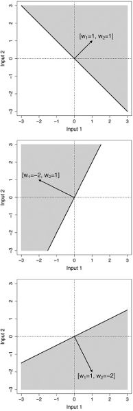
Figure 3.5 Decision boundaries for a two-input neuron. Top: weight vector [w1=1, w2=1]; middle: weight vector [w1=-2, w2=1]; bottom: weight vector [w1=1, w2=-2]. The weights used to create each plot change from one plot to the next. These changes are reflected in the direction of the arrow (the weight vector) in each plot. Specifically, changing the weights rotates the weight vector around the origin. Notice that the decision boundary in each plot is sensitive to the direction of the weight vector: in all the plots, the decision boundary is orthogonal (i.e., at a right, or 90°, angle) to the weight vector. So, changing the weights not only rotates the weight vector, it also rotates the decision boundary of the neuron. This rotation changes the set of inputs that the neuron outputs a high activation in response to (the gray regions).
To understand why this decision boundary is always orthogonal to the weight vector, we have to shift our perspective, for a moment, to linear algebra. Remember that every point in the input space defines a potential combination of input values to the neuron. Now, imagine each of these sets of input values as defining an arrow from the origin to the coordinates of the point in the input space. There is one arrow for each point in the input space. Each of these arrows is very similar to the weight vector, except that it points to the coordinates of the inputs rather than to the coordinates of the weights. When we treat a set of inputs as a vector, the weighted sum calculation is the same as multiplying two vectors, the input vector by the weight vector. In linear algebra terminology, multiplying two vectors is known as the dot product operation. For the purposes of this discussion, all we need to know about the dot product is that the result of this operation is dependent on the angle between the two vectors that are multiplied. If the angle between the two vectors is less than a right angle, then the result will be positive; otherwise, it will be negative. So, multiplying the weight vector by an input vector will return a positive value for all the input vectors at an angle less than a right angle to the weight vector, and a negative value for all the other vectors. The activation function used by this neuron returns a high activation when positive values are input and a low activation when negative values are input. Consequently, the decision boundary lies at a right angle to the weight vector because all the inputs at an angle less than a right angle to the weight vector will result in a positive input to the activation function and, therefore, trigger a high-output activation from the neuron; conversely, all the other inputs will result in a low-output activation from the neuron.
Switching back to the plots in figure 3.5, although the decision boundaries in each of the plots are at different angles, all the decision boundaries go through the point in space that the weight vectors originate from (i.e., the origin). This illustrates that changing the weights of a neuron rotates the neuron’s decision boundary but does not translate it. Translating the decision boundary means moving the decision boundary up and down the weight vector, so that the point where it meets the vector is not the origin. The restriction that all decision boundaries must pass through the origin limits the distinctions that a neuron can learn between input patterns. The standard way to overcome this limitation is to extend the weighted sum calculation so that it includes an extra element, known as the bias term. This bias term is not the same as the inductive bias we discussed in chapter 1. It is more analogous to the intercept parameter in the equation of a line, which moves the line up and down the y-axis. The purpose of this bias term is to move (or translate) the decision boundary away from the origin.
The bias term is simply an extra value that is included in the calculation of the weighted sum. It is introduced into the neuron by adding the bias to the result of the weighted summation prior to passing it through the activation function. Here is the equation describing the processing stages in a neuron with the bias term represented by the term b:

Figure 3.6 illustrates how the value of the bias term affects the decision boundary of a neuron. When the bias term is negative, the decision boundary is moved away from the origin in the direction that the weight vector points to (as in the top and middle plots in figure 3.6); when the bias term is positive, the decision boundary is translated in the opposite direction (see the bottom plot of figure 3.6). In both cases, the decision boundary remains orthogonal to the weight vector. Also, the size of the bias term affects the amount the decision boundary is moved from the origin; the larger the value of the bias term, the more the decision boundary is moved (compare the top plot of figure 3.6 with the middle and bottom plots).
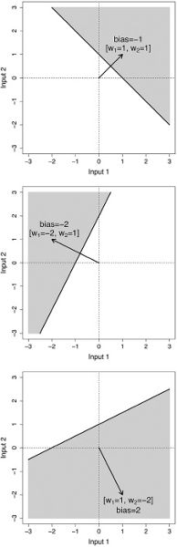
Figure 3.6 Decision boundary plots for a two-input neuron that illustrate the effect of the bias term on the decision boundary. Top: weight vector [w1=1, w2=1] and bias equal to -1; middle: weight vector [w1=-2, w2=1] and bias equal to -2; bottom: weight vector [w1=1, w2=-2] and bias equal to 2. Instead of manually setting the value of the bias term, it is preferable to allow a neuron to learn the appropriate bias. The simplest way to do this is to treat the bias term as a weight and allow the neuron to learn the bias term at the same time that it is learning the rest of the weights for its inputs. All that is required to achieve this is to augment all the input vectors the neuron receives with an extra input that is always set to 1. By convention, this input is input 0 (
), and, consequently, the bias term is specified by weight 0 (
).2 Figure 3.7 illustrates the structure of an artificial neuron when the bias term has been integrated as
.
When the bias term has been integrated into the weights of a neuron, the equation specifying the mapping from input(s) to output activation of the neuron can be simplified (at least from a notational perspective) as follows:
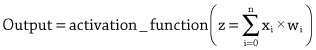
Notice that in this equation the index
goes from
to
, so that it now includes the fixed input,
, and the bias term,
; in the earlier version of this equation, the index only went from
to
. This new format means that the neuron is able to learn the bias term, simply by learning the appropriate weight
, using the same process that is used to learn the weights for the other inputs: at the start of training, the bias term for each neuron in the network will be initialized to a random value and then adjusted, along with the weights of the network, in response to the performance of the network on the dataset.
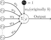
Figure 3.7 An artificial neuron with a bias term included as w0. Accelerating Neural Network Training Using GPUs
Merging the bias term is more than a notational convenience; it enables us to use specialized hardware to accelerate the training of neural networks. The fact that a bias term can be treated as the same as a weight means that the calculation of the weighted sum of inputs (including the addition of the bias term) can be treated as the multiplication of two vectors. As we discussed earlier, during the explanation of why the decision boundary was orthogonal to the weight vector, we can think of a set of inputs as a vector. Recognizing that much of the processing within a neural network involves vector and matrix multiplications opens up the possibility of using specialized hardware to speed up these calculations. For example, graphics processing units (GPUs) are hardware components that have specifically been designed to do extremely fast matrix multiplications.
In a standard feedforward network, all the neurons in one layer receive all the outputs (i.e., activations) from all the neurons in the preceding layer. This means that all the neurons in a layer receive the same set of inputs. As a result, we can calculate the weighted sum calculation for all the neurons in a layer using only a single vector by matrix multiplication. Doing this is much faster than calculating a separate weighted sum for each neuron in the layer. To do this calculation of weighted sums for an entire layer of neurons in a single multiplication, we put the outputs from the neurons in the preceding layer into a vector and store all the weights of the connections between the two layers of neurons in a matrix. We then multiply the vector by the matrix, and the resulting vector contains the weighted sums for all the neurons.
Figure 3.8 illustrates how the weighted summation calculations for all the neurons in a layer in a network can be calculated using a single matrix multiplication operation. This figure is composed of two separate graphics: the graphic on the left illustrates the connections between neurons in two layers of a network, and the graphic on the right illustrates the matrix operation to calculate the weighted sums for the neurons in the second layer of the network. To help maintain a correspondence between the two graphics, the connections into neuron E are highlighted in the graphic on the left, and the calculation of the weighted sum in neuron E is highlighted in the graphic on the right.
Focusing on the graphic on the right, the
vector (1 row, 3 columns) on the bottom-left of this graphic, stores the activations for the neurons in layer 1 of the network; note that these activations are the outputs from an activation function
(the particular activation function is not specified—it could be a threshold function, a tanh, a logistic function, or a rectified linear unit/ReLU function). The
matrix (three rows and four columns), in the top-right of the graphic, holds the weights for the connections between the two layers of neurons. In this matrix, each column stores the weights for the connections coming into one of the neurons in the second layer of the network. The first column stores the weights for neuron D, the second column for neuron E, etc.3 Multiplying the
vector of activations from layer 1 by the
weight matrix results in a
vector corresponding to the weighted summations for the four neurons in layer 2 of the network:
is the weighted sum of inputs for neuron D,
for neuron E, and so on.
To generate the
vector containing the weighted summations for the neurons in layer 2, the activation vector is multiplied by each column in the matrix in turn. This is done by multiplying the first (leftmost) element in the vector by the first (topmost) element in the column, then multiplying the second element in the vector by the element in the second row in the column, and so on, until each element in the vector has been multiplied by its corresponding column element. Once all the multiplications between the vector and the column have been completed, the results are summed together and the stored in the output vector. Figure 3.8 illustrates multiplication of the activation vector by the second column in the weight matrix (the column containing the weights for inputs to neuron E) and the storing of the summation of these multiplications in the output vector as the value
.
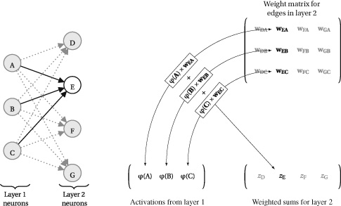
Figure 3.8 A graphical illustration of the topological connections of a specific neuron E in a network, and the corresponding vector by matrix multiplication that calculates the weighted summation of inputs for the neuron E, and its siblings in the same layer.5 Indeed, the calculation implemented by an entire neural network can be represented as a chain of matrix multiplications, with an element-wise application of activation functions to the results of each multiplication. Figure 3.9 illustrates how a neural network can be represented in both graph form (on the left) and as a sequence of matrix operations (on the right). In the matrix representation, the
symbol represents standard matrix multiplication (described above) and the
notation represents the application of an activation function to each element in the vector created by the preceding matrix multiplication. The output of this element-wise application of the activation function is a vector containing the activations for the neurons in a layer of the network. To help show the correspondence between the two representations, both figures show the inputs to the network,
and
, the activations from the three hidden units,
,
, and
, and the overall output of the network,
.

Figure 3.9 A graph representation of a neural network (left), and the same network represented as a sequence of matrix operations (right).6 As a side note, the matrix representation provides a transparent view of the depth of a network; the network’s depth is counted as the number of layers that have a weight matrix associated with them (or equivalently, the depth of a network is the number of weight matrices required by the network). This is why the input layer is not counted when calculating the depth of a network: it does not have a weight matrix associated with it.
As mentioned above, the fact that the majority of calculations in a neural network can be represented as a sequence of matrix operations has important computational implications for deep learning. A neural network may contain over a million neurons, and the current trend is for the size of these networks to double every two to three years.4 Furthermore, deep learning networks are trained by iteratively running a network on examples sampled from very large datasets and then updating the network parameters (i.e., the weights) to improve performance. Consequently, training a deep learning network can require very large numbers of network runs, with each network run requiring millions of calculations. This is why computational speedups, such as those that can be achieved by using GPUs to perform matrix multiplications, have been so important for the development of deep learning.
The relationship between GPUs and deep learning is not one-way. The growth in demand for GPUs generated by deep learning has had a significant impact on GPU manufacturers. Deep learning has resulted in these companies refocusing their business. Traditionally, these companies would have focused on the computer games market, since the original motivation for developing GPU chips was to improve graphics rendering, and this had a natural application to computer games. However, in recent years these companies have focused on positioning GPUs as hardware for deep learning and artificial intelligence applications. Furthermore, GPU companies have also invested to ensure that their products support the top deep learning software frameworks.
Summary
The primary theme in this chapter has been that deep learning networks are composed of large numbers of simple processing units that work together to learn and implement complex mappings from large datasets. These simple units, neurons, execute a two-stage process: first, a weighted summation over the inputs to the neuron is calculated, and second, the result of the weighted summation is passed through a nonlinear function, known as an activation function. The fact that a weighted summation function can be efficiently calculated across a layer of neurons using a single matrix multiplication operation is important: it means that neural networks can be understood as a sequence of matrix operations; this has permitted the use of GPUs, hardware optimized to perform fast matrix multiplication, to speed up the training of networks, which in turn has enabled the size of networks to grow.
The compositional nature of neural networks means that it is possible to understand at a very fundamental level how a neural network operates. Providing a comprehensive description of this level of processing has been the focus of this chapter. However, the compositional nature of neural networks also raises a raft of questions in relation to how a network should be composed to solve a given task, for example:
• Which activation functions should the neurons in a network use?
• How many layers should there be in a network?
• How many neurons should there be in each layer?
• How should the neurons be connected together?Unfortunately, many of these questions cannot be answered at a level of pure principle. In machine learning terminology, the types of concepts these questions are about are known as hyperparameters, as distinct from model parameters. The parameters of a neural network are the weights on the edges, and these are set by training the network using large datasets. By contrast, hyperparameters are the parameters of a model (in these cases, the parameters of a neural network architecture) and/or training algorithm that cannot be directly estimated from the data but instead must be specified by the person creating the model, either through the use of heuristic rules, intuition, or trial and error. Often, much of the effort that goes into the creation of a deep learning network involves experimental work to answer the questions in relation to hyperparameters, and this process is known as hyperparameter tuning. The next chapter will review the history and evolution of deep learning, and the challenges posed by many of these questions are themes running through the review. Subsequent chapters in the book will explore how answering these questions in different ways can create networks with very different characteristics, each suited to different types of tasks. For example, recurrent neural networks are best suited to processing sequential/time-series data, whereas convolutional neural networks were originally developed to process images. Both of these network types are, however, built using the same fundamental processing unit, the artificial neuron; the differences in the behavior and abilities of these networks stems from how these neurons are arranged and composed.
4 A Brief History of Deep Learning
The history of deep learning can be described as three major periods of excitement and innovation, interspersed with periods of disillusionment. Figure 4.1 shows a timeline of this history, which highlights these periods of major research: on threshold logic units (early 1940s to the mid 1960s), connectionism (early 1980s to mid-1990s), and deep learning (mid 2000s to the present). Figure 4.1 distinguishes some of the primary characteristics of the networks developed in each of these three periods. The changes in these network characteristics highlight some of the major themes within the evolution of deep learning, including: the shift from binary to continuous values; the move from threshold activation functions, to logistic and tanh activation, and then onto ReLU activation; and the progressive deepening of the networks, from single layer, to multiple layer, and then onto deep networks. Finally, the upper half of figure 4.1 presents some of the important conceptual breakthroughs, training algorithms, and model architectures that have contributed to the evolution of deep learning.
Figure 4.1 provides a map of the structure of this chapter, with the sequence of concepts introduced in the chapter generally following the chronology of this timeline. The two gray rectangles in figure 4.1 represent the development of two important deep learning network architectures: convolutional neural networks (CNNs), and recurrent neural networks (RNNs). We will describe the evolution of these two network architectures in this chapter, and chapter 5 will give a more detailed explanation of how these networks work.
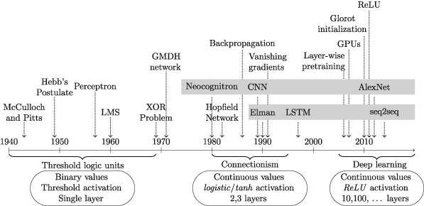
Figure 4.1 History of Deep Learning. Early Research: Threshold Logic Units
In some of the literature on deep learning, the early neural network research is categorized as being part of cybernetics, a field of research that is concerned with developing computational models of control and learning in biological units. However, in figure 4.1, following the terminology used in Nilsson (1965), this early work is categorized as research on threshold logic units because this term transparently describes the main characteristics of the systems developed during this period. Most of the models developed in the 1940s, ’50s, and ’60s processed Boolean inputs (true/false represented as +1/-1 or 1/0) and generated Boolean outputs. They also used threshold activation functions (introduced in chapter 3), and were restricted to single-layer networks; in other words, they were restricted to a single matrix of tunable weights. Frequently, the focus of this early research was on understanding whether computational models based on artificial neurons had the capacity to learn logical relations, such as conjunction or disjunction.
In 1943, Walter McCulloch and Walter Pitts published an influential computational model of biological neurons in a paper entitled: “A Logical Calculus of the Ideas Immanent in Nervous Activity” (McCulloch and Pitts 1943). The paper highlighted the all-or-none characteristic of neural activity in the brain and set out to mathematically describe neural activity in terms of a calculus of propositional logic. In the McCulloch and Pitts model, all the inputs and the output to a neuron were either 0 or 1. Furthermore, each input was either excitatory (having a weight of +1) or inhibitory (having a weight of -1). A key concept introduced in the McCulloch and Pitts model was a summation of inputs followed by a threshold function being applied to the result of the summation. In the summation, if an excitatory input was on, it added 1; if an inhibitory input was on, it subtracted 1. If the result of the summation was above a preset threshold, then the output of the neuron was 1; otherwise, it output a 0. In the paper, McCulloch and Pitts demonstrated how logical operations (such as conjunction, disjunction, and negation) could be represented using this simple model. The McCulloch and Pitts model integrated the majority of the elements that are present in the artificial neurons introduced in chapter 3. In this model, however, the neuron was fixed; in other words the weights and threshold were set by han.
In 1949, Donald O. Hebb published a book entitled The Organization of Behavior, in which he set out a neuropsychological theory (integrating psychology and the physiology of the brain) to explain general human behavior. The fundamental premise of the theory was that behavior emerged through the actions and interactions of neurons. For neural network research, the most important idea in this book was a postulate, now known as Hebb’s postulate, which explained the creation of lasting memory in animals based on a process of changes to the connections between neurons:
When an axon of a cell A is near enough to excite a cell B and repeatedly or persistently takes part in firing it, some growth process or metabolic change takes place in one or both cells such that A’s efficiency, as one of the cells firing B, is increased. (Hebb 1949, p. 62)This postulate was important because it asserted that information was stored in the connections between neurons (i.e., in the weights of a network), and furthermore that learning occurred by changing these connections based on repeated patterns of activation (i.e., learning can take place within a network by changing the weights of the network).
Rosenblatt’s Perceptron Training Rule
In the years following Hebb’s publication, a number of researchers proposed computational models of neuron activity that integrated the Boolean threshold activation units of McCulloch and Pitts, with a learning mechanism based on adjusting the weights applied to the inputs. The best known of these models was Frank Rosenblatt’s perceptron model (Rosenblatt 1958). Conceptually, the perceptron model can be understood as a neural network consisting of a single artificial neuron that uses a threshold activation unit. Importantly, a perceptron network only has a single layer of weights. The first implementation of a perceptron was a software implementation on an IBM 704 system (and this was probably the first implementation of any neural network). However, Rosenblatt always intended the perceptron to be a physical machine and it was later implemented in custom-built hardware known as the “Mark 1 perceptron.” The Mark 1 perceptron received input from a camera that generated a 400-pixel image that was passed into the machine via an array of 400 photocells that were in turn connected to the neurons. The weights on connections to the neurons were implemented using adjustable electrical resistors known as potentiometers, and weight adjustments were implemented by using electric motors to adjust the potentiometers.
Rosenblatt proposed an error-correcting training procedure for updating the weights of a perceptron so that it could learn to distinguish between two classes of input: inputs for which the perceptron should produce the output
, and inputs for which the perceptron should produce the output
(Rosenblatt 1960). The training procedure assumes a set of Boolean encoded input patterns, each with an associated target output. At the start of training, the weights in the perceptron are initialized to random values. Training then proceeds by iterating through the training examples, and after each example has been presented to the network, the weights of the network are updated based on the error between the output generated by the perceptron and the target output specified in the data. The training examples can be presented to the network in any order and examples may be presented multiple times before training is completed. A complete training pass through the set of examples is known as an iteration, and training terminates when the perceptron correctly classifies all the examples in an iteration.
Rosenblatt defined a learning rule (known as the perceptron training rule) to update each weight in a perceptron after a training example has been processed. The strategy the rule used to update the weights is the same as the three-condition strategy we introduced in chapter 2 to adjust the weights in the loan decision model:
1. If the output of the model for an example matches the output specified for that example in the dataset, then don’t update the weights.
2. If the output of the model is too low for the current example, then increase the output of the model by increasing the weights for the inputs that had positive value for the example and decreasing the weights for the inputs that had a negative value for the example.
3. If the output of the model is too high for the current example, then reduce the output of the model by decreasing the weights for the inputs that had a positive value and increasing the weights for the inputs that had a negative value for the example.Written out in an equation, Rosenblatt’s learning rule updates a weight
(
) as: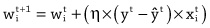
In this rule,
is the value of weight i after the network weights have been updated in response to the processing of example t,
is the value of weight i used during the processing of example t,
is a preset positive constant (known as the learning rate, discussed below),
is the expected output for example t as specified in the training dataset,
is the output generated by the perceptron for example t, and
is the component of input t that was weighted by
during the processing of the example.
Although it may look complex, the perceptron training rule is in fact just a mathematical specification of the three-condition weight update strategy described above. The primary part of the equation to understand is the calculation of the difference between the expected output and what the perceptron actually predicted:
. The outcome of this subtraction tells us which of the three update conditions we are in. In understanding how this subtraction works, it is important to remember that for a perceptron model the desired output is always either
or
. The first condition is when
; then the output of the perceptron is correct and the weights are not changed.
The second weight update condition is when the output of the perceptron is too large. This condition can only be occur when the correct output for example
is
and so this condition is triggered when
. In this case, if the perceptron output for the example
is
, then the error term is negative (
) and the weight
is updated by
. Assuming, for the purpose of this explanation, that
is set to 0.5, then this weight update simplifies to
. In other words, when the perceptron’s output is too large, the weight update rule subtracts the input values from the weights. This will decrease the weights on inputs with positive values for the example, and increase the weights on inputs with negative values for the example (subtracting a negative number is the same as adding a positive number).
The third weight update condition is when the output of the perceptron is too small. This weight update condition is the exact opposite of the second. It can only occur when
and so is triggered when
. In this case (
), and the weight is updated by
. Again assuming that
is set to 0.5, then this update simplifies to
, which highlights that when the error of the perceptron is positive, the rule updates the weight by adding the input to the weight. This has the effect of decreasing the weights on inputs with negative values for the example and increasing the weight on inputs with positive values for the example.
At a number of points in the preceding paragraphs we have referred to learning rate,
. The purpose of the learning rate,
, is to control the size of the adjustments that are applied to a weight. The learning rate is an example of a hyperparameter that is preset before the model is trained. There is a tradeoff in setting the learning rate:
• If the learning rate is too small, it may take a very long time for the training process to converge on an appropriate set of weights.
• If the learning rate is too large, the network’s weights may jump around the weight space too much and the training may not converge at all.One strategy for setting the learning rate is to set it to a relatively small positive value (e.g., 0.01), and another strategy is to initialize it to a larger value (e.g., 1.0) but to systematically reduce it as the training progresses
(e.g.,

).
To make this discussion regarding the learning rate more concrete, imagine you are trying to solve a puzzle that requires you to get a small ball to roll into a hole. You are able to control the direction and speed of the ball by tilting the surface that the ball is rolling on. If you tilt the surface too steeply, the ball will move very fast and is likely to go past the hole, requiring you to adjust the surface again, and if you overadjust you may end up repeatedly tilting the surface. On the other hand, if you only tilt the surface a tiny bit, the ball may not start to move at all, or it may move very slowly taking a long time to reach the hole. Now, in many ways the challenge of getting the ball to roll into the hole is similar to the problem of finding the best set of weights for a network. Think of each point on the surface the ball is rolling across as a possible set of network weights. The ball’s position at each point in time specifies the current set of weights of the network. The position of the hole specifies the optimal set of network weights for the task we are training the network to complete. In this context, guiding the network to the optimal set of weights is analogous to guiding the ball to the hole. The learning rate allows us to control how quickly we move across the surface as we search for the optimal set of weights. If we set the learning rate to a high value, we move quickly across the surface: we allow large updates to the weights at each iteration, so there are big differences between the network weights in one iteration and the next. Or, using our rolling ball analogy, the ball is moving very quickly, and just like in the puzzle when the ball is rolling too fast and passes the hole, our search process may be moving so fast that it misses the optimal set of weights. Conversely, if we set the learning rate to a low value, we move very slowly across the surface: we only allow small updates to the weights at each iteration; or, in other words, we only allow the ball to move very slowly. With a low learning rate, we are less likely to miss the optimal set of weights, but it may take an inordinate amount of time to get to them. The strategy of starting with a high learning rate and then systematically reducing it is equivalent to steeply tilting the puzzle surface to get the ball moving and then reducing the tilt to control the ball as it approaches the hole.
Rosenblatt proved that if a set of weights exists that enables the perceptron to properly classify all of the training examples correctly, the perceptron training algorithm will eventually converge on this set of weights. This finding is known as the perceptron convergence theorem (Rosenblatt 1962). The difficulty with training a perceptron, however, is that it may require a substantial number of iterations through the data before the algorithm converges. Furthermore, for many problems it is unknown whether an appropriate set of weights exists in advance; consequently, if training has been going on for a long time, it is not possible to know whether the training process is simply taking a long time to converge on the weights and terminate, or whether it will never terminate.
The Least Mean Squares Algorithm
Around the same time that Rosenblatt was developing the perceptron, Bernard Widrow and Marcian Hoff were developing a very similar model called the ADALINE (short for adaptive linear neuron), along with a learning rule called the LMS (least mean square) algorithm (Widrow and Hoff 1960). An ADALINE network consists of a single neuron that is very similar to a perceptron; the only difference is that an ADALINE network does not use a threshold function. In fact, the output of an ADALINE network is the just the weighted sum of the inputs. This is why it is known as a linear neuron: a weighted sum is a linear function (it defines a line), and so an ADALINE network implements a linear mapping from inputs to output. The LMS rule is nearly identical to the perceptron learning rule, except that the output of the perceptron for a given example
is replaced by the weighted sum of the inputs:
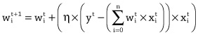
The logic of the LMS update rule is the same as that of the perceptron training rule. If the output is too large, then weights that were applied to a positive input caused the output to be larger, and these weights should be decreased, and those that were applied to a negative input should be increased, thereby reducing the output the next time this input pattern is received. And, by the same logic, if the output is too small, then weights that were applied to a positive input are increased and those that were applied to a negative input should be decreased.
If the output of the model is too large, then weights associated with positive inputs should be reduced, whereas if the output is too small, then these weights should be increased.
One of the important aspects of Widrow and Hoff’s work was to show that LMS rule could be used to train network to predict a number of any value, not just a +1 or -1. This learning rule was called the least mean square algorithm because using the LMS rule to iteratively adjust the weights in a neuron is equivalent to minimizing the average squared error on the training set. Today, the LMS learning rule is sometimes called the Widrow-Hoff learning rule, after the inventors; however, it is more commonly called the delta rule because it uses the difference (or delta) between desired output and the actual output to calculate the weight adjustments. In other words, the LMS rule specifies that a weight should be adjusted in proportion to the difference between the output of an ADALINE network and the desired output: if the neuron makes a large error, then the weights are adjusted by a large amount, if the neuron makes a small error, then weights are adjusted by a small amount.
Today, the perceptron is recognized as important milestone in the development of neural networks because it was the first neural network to be implemented. However, most modern algorithms for training neural networks are more similar to the LMS algorithm. The LMS algorithm attempts to minimize the mean squared error of the network. As will be discussed in chapter 6, technically this iterative error reduction process involves a gradient descent down an error surface; and, today, nearly all neural networks are trained using some variant of gradient descent.
The XOR Problem
The success of Rosenblatt, Widrow and Hoff, and others, in demonstrating that neural network models could automatically learn to distinguish between different sets of patterns, generated a lot of excitement around artificial intelligence and neural network research. However, in 1969, Marvin Minsky and Seymour Papert published a book entitled Perceptrons, which, in the annals of neural network research, is attributed with single-handedly destroying this early excitement and optimism (Minsky and Papert 1969). Admittedly, throughout the 1960s neural network research had suffered from a lot of hype, and a lack of success in terms of fulfilling the correspondingly high expectations. However, Minsky and Papert’s book set out a very negative view of the representational power of neural networks, and after its publication funding for neural network research dried up.
Minsky and Papert’s book primarily focused on single layer perceptrons. Remember that a single layer perceptron is the same as a single neuron that uses a threshold activation function, and so a single layer perceptron is restricted to implementing a linear (straight-line) decision boundary.1 This means that a single layer perceptron can only learn to distinguish between two classes of inputs if it is possible to draw a straight line in the input space that has all of the examples of one class on one side of the line and all examples of the other class on the other side of the line. Minsky and Papert highlighted this restriction as a weakness of these models.
To understand Minsky and Papert’s criticism of single layer perceptrons, we must first understand the concept of a linearly separable function. We will use a comparison between the logical AND and OR functions with the logical XOR function to explain the concept of a linearly separable function. The AND function takes two inputs, each of which can be either TRUE or FALSE, and returns TRUE if both inputs are TRUE. The plot on the left of figure 4.4 shows the input space for the AND function and categorizes each of the four possible input combinations as either resulting in an output value of TRUE (shown in the figure by using a clear dot) or FALSE (shown in the figure by using black dots). This plot illustrates that is possible to draw a straight line between the inputs for which the AND function returns TRUE, (T,T), and the inputs for which the function returns FALSE, {(F,F), (F,T), (T,F)}. The OR function is similar to the AND function, except that it returns TRUE if either or both inputs are TRUE. The middle plot in figure 4.4 shows that it is possible to draw a line that separates the inputs that the OR function classifies as TRUE, {(F,T), (T,F), (T,T)}, from those it classifies as FALSE, (F,F). It is because we can draw a single straight line in the input space of these functions that divides the inputs belonging to one category of output from the inputs belonging to the other output category that the AND and OR functions are linearly separable functions.
The XOR function is also similar in structure to the AND and OR functions; however, it only returns TRUE if one (but not both) of its inputs are TRUE. The plot on the right of figure 4.2 shows the input space for the XOR function and categorizes each of the four possible input combinations as returning either TRUE (shown in the figure by using a clear dot) or FALSE (shown in the figure by using black dots). Looking at this plot you will see that it is not possible to draw a straight line between the inputs the XOR function classifies as TRUE and those that it classifies as FALSE. It is because we cannot use a single straight line to separate the inputs belonging to different categories of outputs for the XOR function that this function is said to be a nonlinearly separable function. The fact that the XOR function is nonlinearly separable does not make the function unique, or even rare—there are many functions that are nonlinearly separable.
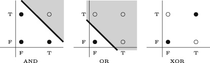
Figure 4.2 Illustrations of the linearly separable function. In each figure, black dots represent inputs for which the function returns FALSE, circles represent inputs for which the function returns TRUE. (T stands for true and F stands for false.) The key criticism that Minsky and Papert made of single layer perceptrons was that these single layer models were unable to learn nonlinearly separable functions, such as the XOR function. The reason for this limitation is that the decision boundary of a perceptron is linear and so a single layer perceptron cannot learn to distinguish between the inputs that belong to one output category of a nonlinearly separable function from those that belong to the other category.
It was known at the time of Minsky and Papert’s publication that it was possible to construct neural networks that defined a nonlinear decision boundary, and thus learn nonlinearly separable functions (such as the XOR function). The key to creating networks with more complex (nonlinear) decision boundaries was to extend the network to have multiple layers of neurons. For example, figure 4.3 shows a two-layer network that implements the XOR function. In this network, the logical TRUE and FALSE values are mapped to numeric values: FALSE values are represented by 0, and TRUE values are represented by 1. In this network, units activate (output +1) if the weighted sum of inputs is
; otherwise, they output 0. Notice that the units in the hidden layer implement the logical AND and OR functions. These can be understood as intermediate steps to solving the XOR challenge. The unit in the output layer implements the XOR by composing the outputs of these hidden layers. In other words, the unit in the output layer returns TRUE only when the AND node is off (output=0) and the OR node is on (output=1). However, it wasn’t clear at the time how to train networks with multiple layers. Also, at the end of their book, Minsky and Papert argued that “in their judgment” the research on extending neural networks to multiple layers was “sterile” (Minsky and Papert 1969, sec. 13.2 page 23).
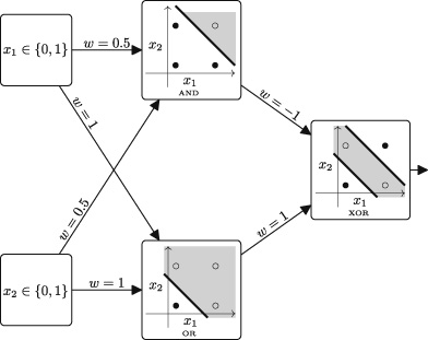
Figure 4.3 A network that implements the XOR function. All processing units use a threshold activation function with a threshold of ≥1. In a somewhat ironic historical twist, contemporaneous with Minsky and Papert’s publication, Alexey Ivakhnenko, a Ukrainian researcher, proposed the group method for data handling (GMDH), and in 1971 published a paper that described how it could be used to learn a neural network with eight layers (Ivakhnenko 1971). Today Ivakhnenko’s 1971 GMDH network is credited with being the first published example of a deep network trained from data (Schmidhuber 2015). However, for many years, Ivaknenko’s accomplishment was largely overlooked by the wider neural network community. As a consequence, very little of the current work in deep learning uses the GMDH method for training: in the intervening years other training algorithms, such as backpropagation (described below), became standardized in the community. At the same time of Ivakhnenko’s overlooked accomplishment, Minsky and Papert’s critique was proving persuasive and it heralded the end of the first period of significant research on neural networks.
This first period of neural network research, did, however, leave a legacy that shaped the development of the field up to the present day. The basic internal structure of an artificial neuron was defined: a weighted sum of inputs fed through an activation function. The concept of storing information within the weights of a network was developed. Furthermore, learning algorithms based on iteratively adapting weights were proposed, along with practical learning rules, such as the LMS rule. In particular, the LMS approach, of adjusting the weights of neurons in proportion to the difference between the output of the neuron and the desired output, is present in most modern training algorithms. Finally, there was recognition of the limitations of single layer networks, and an understanding that one way to address these limitations was to extend the networks to include multiple layers of neurons. At this time, however, it was unclear how to train networks with multiple layers. Updating a weight requires an understanding of how the weight affects the error of the network. For example, in the LMS rule if the output of the neuron was too large, then weights that were applied to positive inputs caused the output to increase. Therefore, decreasing the size of these weight would reduce the output and thereby reduce the error. But, in the late 1960s, the question of how to model the relationship between the weights of the inputs to neurons in the hidden layers of a network and the overall error of the network was still unanswered; and, without this estimation of the contribution of the weight to the error, it was not possible to adjust the weights in the hidden layers of a network. The problem of attributing (or assigning) an amount of error to the components in a network is sometimes referred to as the credit assignment problem, or as the blame assignment problem.
Connectionism: Multilayer Perceptrons
In the 1980s, people began to reevaluate the criticisms of the late 1960s as being overly severe. Two developments, in particular, reinvigorated the field: (1) Hopfield networks; and (2) the backpropagation algorithm.
In 1982, John Hopfield published a paper where he described a network that could function as an associative memory (Hopfield 1982). During training, an associative memory learns a set of input patterns. Once the associate memory network has been trained, then, if a corrupted version of one of the input patterns is presented to the network, the network is able to regenerate the complete correct pattern. Associative memories are useful for a number of tasks, including pattern completion and error correction. Table 4.12 illustrates the tasks of pattern completion and error correction using the example of an associative memory that has been trained to store information on people’s birthdays. In a Hopfield network, the memories, or input patterns, are encoded in binary strings; and, assuming binary patterns are relatively distinct from each other, a Hopfield network can store up to 0.138N of these strings, where N is the number of neurons in the network. So to store 10 distinct patterns requires a Hopfield network with 73 neurons, and to store 14 distinct patterns requires 100 neurons.
Table 4.1. Illustration of the uses of an association memory for pattern completion and error correction
Training patterns Pattern completion John**12MayLiz***?????→ Liz***25FebKerry*03Jan???***10Mar→ Des***10MarLiz***25FebError correction Des***10MarKerry*01Apr→ Kerry*03JanJosef*13DecJxsuf*13Dec→ Josef*13DecBackpropagation and Vanishing Gradients
In 1986, a group of researchers known as the parallel distributed processing (PDP) research group published a two-book overview of neural network research (Rumelhart et al. 1986b, 1986c). These books proved to be incredibly popular, and chapter 8 in volume one described the backpropagation algorithm (Rumelhart et al. 1986a). The backpropagation algorithm has been invented a number of times,3 but it was this chapter by Rumelhart, Hinton, and Williams, published by PDP, that popularized its use. The backpropagation algorithm is a solution to the credit assignment problem and so it can be used to train a neural network that has hidden layers of neurons. The backpropagation algorithm is possibly the most important algorithm in deep learning. However, a clear and complete explanation of the backpropagation algorithm requires first explaining the concept of an error gradient, and then the gradient descent algorithm. Consequently, the in-depth explanation of backpropagation is postponed until chapter 6, which begins with an explanation of these necessary concepts. The general structure of the algorithm, however, can be described relatively quickly. The backpropagation algorithm starts by assigning random weights to each of the connections in the network. The algorithm then iteratively updates the weights in the network by showing training instances to the network and updating the network weights until the network is working as expected. The core algorithm works in a two-stage process. In the first stage (known as the forward pass), an input is presented to the network and the neuron activations are allowed to flow forward through the network until an output is generated. The second stage (known as the backward pass) begins at the output layer and works backward through the network until the input layer is reached. This backward pass begins by calculating an error for each neuron in the output layer. This error is then used to update the weights of these output neurons. Then the error of each output neuron is shared back (backpropagated) to the hidden neurons that connect to it, in proportion to the weights on the connections between the output neuron and the hidden neuron. Once this sharing (or blame assignment) has been completed for a hidden neuron, the total blame attributable to that hidden neuron is summed and this total is used to update the weights on that neuron. The backpropagation (or sharing back) of blame is then repeated for the neurons that have not yet had blame attributed to them. This process of blame assignment and weight updates continues back through the network until all the weights have been updated.
A key innovation that enabled the backpropagation algorithm to work was a change in the activation functions used in the neurons. The networks that were developed in the early years of neural network research used threshold activation functions. The backpropagation algorithm does not work with threshold activation functions because backpropagation requires that the activation functions used by the neurons in the network be differentiable. Threshold activation functions are not differentiable because there is a discontinuity in the output of the function at the threshold. In other words, the slope of a threshold function at the threshold is infinite and therefore it is not possible to calculate the gradient of the function at that point. This led to the use of differentiable activation functions in multilayer neural networks, such as the logistic and tanh functions.
There is, however, an inherent limitation with using the backpropagation algorithm to train deep networks. In the 1980s, researchers found that backpropagation worked well with relatively shallow networks (one or two layers of hidden units), but that as the networks got deeper, the networks either took an inordinate amount of time to train, or else they entirely failed to converge on a good set of weights. In 1991, Sepp Hochreiter (working with Jürgen Schmidhuber) identified the cause of this problem in his diploma thesis (Hochreiter 1991). The problem is caused by the way the algorithm backpropagates errors. Fundamentally, the backpropagation algorithm is an implementation of the chain rule from calculus. The chain rule involves the multiplication of terms, and backpropagating an error from one neuron back to another can involve multiplying the error by a number terms with values less than 1. These multiplications by values less than 1 happen repeatedly as the error signal gets passed back through the network. This results in the error signal becoming smaller and smaller as it is backpropagated through the network. Indeed, the error signal often diminishes exponentially with respect to the distance from the output layer. The effect of this diminishing error is that the weights in the early layers of a deep network are often adjusted by only a tiny (or zero) amount during each training iteration. In other words, the early layers either train very, very slowly or do not move away from their random starting positions at all. However, the early layers in a neural network are vitally important to the success of the network, because it is the neurons in these layers that learn to detect the features in the input that the later layers of the network use as the fundamental building blocks of the representations that ultimately determine the output of the network. For technical reasons, which will be explained in chapter 6, the error signal that is backpropagated through the network is in fact the gradient of the error of the network, and, as a result, this problem of the error signal rapidly diminishing to near zero is known as the vanishing gradient problem.
Connectionism and Local versus Distributed Representations
Despite the vanishing gradient problem, the backpropagation algorithm opened up the possibility of training more complex (deeper) neural network architectures. This aligned with the principle of connectionism. Connectionism is the idea that intelligent behavior can emerge from the interactions between large numbers of simple processing units. Another aspect of connectionism was the idea of a distributed representation. A distinction can be made in the representations used by neural networks between localist and distributed representations. In a localist representation there is a one-to-one correspondence between concepts and neurons, whereas in a distributed representation each concept is represented by a pattern of activations across a set of neurons. Consequently, in a distributed representation each concept is represented by the activation of multiple neurons and the activation of each neuron contributes to the representation of multiple concepts.
In a distributed representation each concept is represented by the activation of multiple neurons and the activation of each neuron contributes to the representation of multiple concepts.
To illustrate the distinction between localist and distributed representations, consider a scenario where (for some unspecified reason) a set of neuron activations is being used to represent the absence or presence of different foods. Furthermore, each food has two properties, the country of origin of the recipe and its taste. The possible countries of origin are: Italy, Mexico, or France; and, the set of possible tastes are: Sweet, Sour, or Bitter. So, in total there are nine possible types of food: Italian+Sweet, Italian+Sour, Italian+Bitter, Mexican+Sweet, etc. Using a localist representation would require nine neurons, one neuron per food type. There are, however, a number of ways to define a distributed representation of this domain. One approach is to assign a binary number to each combination. This representation would require only four neurons, with the activation pattern 0000 representing Italian+Sweet, 0001 representing Italian+Sour, 0010 representing Italian+Bitter, and so on up to 1000 representing French+Bitter. This is a very compact representation. However, notice that in this representation the activation of each neuron in isolation has no independently meaningful interpretation: the rightmost neuron would be active (***1) for Italian+Sour, Mexican+Sweet, Mexican+Bitter, and France+Sour, and without knowledge of the activation of the other neurons, it is not possible know what country or taste is being represented. However, in a deep network the lack of semantic interpretability of the activations of hidden units is not a problem, so long as the neurons in the output layer of the network are able to combine these representations in such a way so as to generate the correct output. Another, more transparent, distributed representation of this food domain is to use three neurons to represent the countries and three neurons to represent the tastes. In this representation, the activation pattern 100100 could represent Italian+Sweet, 001100 could represent French+Sweet, and 001001 could represent French+Bitter. In this representation, the activation of each neuron can be independently interpreted; however the distribution of activations across the set of neurons is required in order to retrieve the full description of the food (country+taste). Notice, however, that both of these distributed representations are more compact than the localist representation. This compactness can significantly reduce the number of weights required in a network, and this in turn can result in faster training times for the network.
The concept of a distributed representation is very important within deep learning. Indeed, there is a good argument that deep learning might be more appropriately named representation learning—the argument being that the neurons in the hidden layers of a network are learning distributed representations of the input that are useful intermediate representations in the mapping from inputs to outputs that the network is attempting to learn. The task of the output layer of a network is then to learn how to combine these intermediate representations so as to generate the desired outputs. Consider again the network in figure 4.3 that implements the XOR function. The hidden units in this network learn an intermediate representation of the input, which can be understood as composed of the AND and OR functions; the output layer then combines this intermediate representation to generate the required output. In a deep network with multiple hidden layers, each subsequent hidden layer can be interpreted as learning a representation that is an abstraction over the outputs of the preceding layer. It is this sequential abstraction, through learning intermediate representations, that enables deep networks to learn such complex mappings from inputs to outputs.
Network Architectures: Convolutional and Recurrent Neural Networks
There are a considerable number of ways in which a set of neurons can be connected together. The network examples presented so far in the book have been connected together in a relatively uncomplicated manner: neurons are organized into layers and each neuron in a layer is directly connected to all of the neurons in the next layer of the network. These networks are known as feedforward networks because there are no loops within the network connections: all the connections point forward from the input toward the output. Furthermore, all of our network examples thus far would be considered to be fully connected, because each neuron is connected to all the neurons in the next layer. It is possible, and often useful, to design and train networks that are not feedforward and/or that are not fully connected. When done correctly, tailoring network architectures can be understood as embedding into the network architecture information about the properties of the problem that the network is trying to learn to model.
A very successful example of incorporating domain knowledge into a network by tailoring the networks architecture is the design of convolutional neural networks (CNNs) for object recognition in images. In the 1960s, Hubel and Wiesel carried out a series of experiments on the visual cortex of cats (Hubel and Wiesel 1962, 1965). These experiments used electrodes inserted into the brains of sedated cats to study the response of the brain cells as the cats were presented with different visual stimuli. Examples of the stimuli used included bright spots or lines of light appearing at a location in the visual field, or moving across a region of the visual field. The experiments found that different cells responded to different stimuli at different locations in the visual field: in effect a single cell in the visual cortex would be wired to respond to a particular type of visual stimulus occurring within a particular region of the visual field. The region of the visual field that a cell responded to was known as the receptive field of the cell. Another outcome of these experiments was the differentiation between two types of cells: “simple” and “complex.” For simple cells, the location of the stimulus is critical with a slight displacement of the stimulus resulting in a significant reduction in the cell’s response. Complex cells, however, respond to their target stimuli regardless of where in the field of vision the stimulus occurs. Hubel and Wiesel (1965) proposed that complex cells behaved as if they received projections from a large number of simple cells all of which respond to the same visual stimuli but differing in the position of their receptive fields. This hierarchy of simple cells feeding into complex cells results in funneling of stimuli from large areas of the visual field, through a set of simple cells, into a single complex cell. Figure 4.4 illustrates this funneling effect. This figure shows a layer of simple cells each monitoring a receptive field at a different location in the visual field. The receptive field of the complex cell covers the layer of simple cells, and this complex cell activates if any of the simple cells in its receptive field activates. In this way the complex cell can respond to a visual stimulus if it occurs at any location in the visual field.
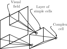
Figure 4.4 The funneling effect of receptive fields created by the hierarchy of simple and complex cells. In the late 1970s and early 1980s, Kunihiko Fukushima was inspired by Hubel and Wiesel’s analysis of the visual cortex and developed a neural network architecture for visual pattern recognition that was called the neocognitron (Fukushima 1980). The design of the neocognitron was based on the observation that an image recognition network should be able to recognize if a visual feature is present in an image irrespective of location in the image—or, to put it slightly more technically, the network should be able to do spatially invariant visual feature detection. For example, a face recognition network should be able to recognize the shape of an eye no matter where in the image it occurs, similar to the way a complex cell in Hubel and Wiesel’s hierarchical model could detect the presence of a visual feature irrespective of where in the visual field it occurred.
Fukushima realized that the functioning of the simple cells in the Hubel and Wiesel hierarchy could be replicated in a neural network using a layer of neurons that all use the same set of weights, but with each neuron receiving inputs from fixed small regions (receptive fields) at different locations in the input field. To understand the relationship between neurons sharing weights and spatially invariant visual feature detection, imagine a neuron that receives a set of pixel values, sampled from a region of an image, as its inputs. The weights that this neuron applies to these pixel values define a visual feature detection function that returns true (high activation) if a particular visual feature (pattern) occurs in the input pixels, and false otherwise. Consequently, if a set of neurons all use the same weights, they will all implement the same visual feature detector. If the receptive fields of these neurons are then organized so that together they cover the entire image, then if the visual feature occurs anywhere in the image at least one of the neurons in the group will identify it and activate.
Fukushima also recognized that the Hubel and Wiesel funneling effect (into complex cells) could be obtained by neurons in later layers also receiving as input the outputs from a fixed set of neurons in a small region of the preceding layer. In this way, the neurons in the last layer of the network each receive inputs from across the entire input field allowing the network to identify the presence of a visual feature anywhere in the visual input.
Some of the weights in neocognitron were set by hand, and others were set using an unsupervised training process. In this training process, each time an example is presented to the network a single layer of neurons that share the same weights is selected from the layers that yielded large outputs in response to the input. The weights of the neurons in the selected layer are updated so as to reinforce their response to that input pattern and the weights of neurons not in the layer are not updated. In 1989 Yann LeCun developed the convolutional neural network (CNN) architecture specifically for the task of image processing (LeCun 1989). The CNN architecture shared many of the design features found in the neocognitron; however, LeCun showed how these types of networks could be trained using backpropagation. CNNs have proved to be incredibly successful in image processing and other tasks. A particularly famous CNN is the AlexNet network, which won the ImageNet Large-Scale Visual Recognition Challenge (ILSVRC) in 2012 (Krizhevsky et al. 2012). The goal of the ILSVRC competition is to identify objects in photographs. The success of AlexNet at the ILSVRC competition generated a lot of excitement about CNNs, and since AlexNet a number of other CNN architectures have won the competition. CNNs are one of the most popular types of deep neural networks, and chapter 5 will provide a more detailed explanation of them.
Recurrent neural networks (RNNs) are another example of a neural network architecture that has been tailored to the specific characteristics of a domain. RNNs are designed to process sequential data, such as language. An RNN network processes a sequence of data (such as a sentence) one input at a time. An RNN has only a single hidden layer. However, the output from each of these hidden neurons is not only fed forward to the output neurons, it is also temporarily stored in a buffer and then fed back into all of the hidden neurons at the next input. Consequently, each time the network processes an input, each neuron in the hidden layer receives both the current input and the output the hidden layer generated in response to the previous input. In order to understand this explanation, it may at this point be helpful to briefly skip forward to figure 5.2 to see an illustration of the structure of an RNN and the flow of information through the network. This recurrent loop, of activations from the output of the hidden layer for one input being fed back into the hidden layer alongside the next input, gives an RNN a memory that enables it to process each input in the context of the previous inputs it has processed.4 RNNs are considered deep networks because this evolving memory can be considered as deep as the sequence is long.
An early well-known RNN is the Elman network. In 1990, Jeffrey Locke Elman published a paper that described an RNN that had been trained to predict the endings of simple two- and three-word utterances (Elman 1990). The model was trained on a synthesized dataset of simple sentences generated using an artificial grammar. The grammar was built using a lexicon of twenty-three words, with each word assigned to a single lexical category (e.g., man=NOUN-HUM, woman=NOUN-HUM, eat=VERB-EAT, cookie=NOUN-FOOD, etc.). Using this lexicon, the grammar defined fifteen sentence generation templates (e.g., NOUN-HUM+VERB-EAT+NOUN-FOOD which would generate sentences such as man eat cookie). Once trained, the model was able to generate reasonable continuations for sentences, such as woman+eat+? = cookie. Furthermore, once the network was started, it was able to generate longer strings consisting of multiple sentences, using the context it generated itself as the input for the next word, as illustrated by this three-sentence example:
girl eat bread dog move mouse mouse move book
Although this sentence generation task was applied to a very simple domain, the ability of the RNN to generate plausible sentences was taken as evidence that neural networks could model linguistic productivity without requiring explicit grammatical rules. Consequently, Elman’s work had a huge impact on psycholinguistics and psychology. The following quote, from Churchland 1996, illustrates the importance that some researchers attributed to Elman’s work:
The productivity of this network is of course a feeble subset of the vast capacity that any normal English speaker commands. But productivity is productivity, and evidently a recurrent network can possess it. Elman’s striking demonstration hardly settles the issue between the rule-centered approach to grammar and the network approach. That will be some time in working itself out. But the conflict is now an even one. I’ve made no secret where my own bets will be placed. (Churchland 1996, p. 143)5Although RNNs work well with sequential data, the vanishing gradient problem is particularly severe in these networks. In 1997, Sepp Hochreiter and Jürgen Schmidhuber, the researchers who in 1991 had presented an explanation of the vanishing gradient problem, proposed the long short-term memory (LSTM) units as a solution to this problem in RNNs (Hochreiter and Schmidhuber 1997). The name of these units draws on a distinction between how a neural network encodes long-term memory (understood as concepts that are learned over a period of time) through training and short-term memory (understood as the response of the system to immediate stimuli). In a neural network, long-term memory is encoded through adjusting the weights of the network and once trained these weights do not change. Short-term memory is encoded in a network through the activations that flow through the network and these activation values decay quickly. LSTM units are designed to enable the short-term memory (the activations) in the network to be propagated over long periods of time (or sequences of inputs). The internal structure of an LSTM is relatively complex, and we will describe it in chapter 5. The fact that LSTM can propagate activations over long periods enables them to process sequences that include long-distance dependencies (interactions between elements in a sequence that are separated by two or more positions). For example, the dependency between the subject and the verb in an English sentence: The dog/dogs in that house is/are aggressive. This has made LSTM networks suitable for language processing, and for a number of years they have been the default neural network architecture for many natural language processing models, including machine translation. For example, the sequence-to-sequence (seq2seq) machine translation architecture introduced in 2014 connects two LSTM networks in sequence (Sutskever et al. 2014). The first LSTM network, the encoder, processes the input sequence one input at a time, and generates a distributed representation of that input. The first LSTM network is called an encoder because it encodes the sequence of words into a distributed representation. The second LSTM network, the decoder, is initialized with the distributed representation of the input and is trained to generate the output sequence one element at a time using a feedback loop that feeds the most recent output element generated by the network back in as the input for the next time step. Today, this seq2seq architecture is the basis for most modern machine translation systems, and is explained in more detail in chapter 5.
By the late 1990s, most of the conceptual requirements for deep learning were in place, including both the algorithms to train networks with multiple layers, and the network architectures that are still very popular today (CNNs and RNNs). However, the problem of the vanishing gradients still stifled the creation of deep networks. Also, from a commercial perspective, the 1990s (similar to the 1960s) experienced a wave of hype based on neural networks and unrealized promises. At the same time, a number of breakthroughs in other forms of machine learning models, such as the development of support vector machines (SVMs), redirected the focus of the machine learning research community away from neural networks: at the time SVMs were achieving similar accuracy to neural network models but were easier to train. Together these factors led to a decline in neural network research that lasted up until the emergence of deep learning.
The Era of Deep Learning
The first recorded use of the term deep learning is credited to Rina Dechter (1986), although in Dechter’s paper the term was not used in relation to neural networks; and the first use of the term in relation to neural networks is credited to Aizenberg et al. (2000).6 In the mid-2000s, interest in neural networks started to grow, and it was around this time that the term deep learning came to prominence to describe deep neural networks. The term deep learning is used to emphasize the fact that the networks being trained are much deeper than previous networks.
One of the early successes of this new era of neural network research was when Geoffrey Hinton and his colleagues demonstrated that it was possible to train a deep neural network using a process known as greedy layer-wise pretraining. Greedy layer-wise pretraining begins by training a single layer of neurons that receives input directly from the raw input. There are a number of different ways that this single layer of neurons can be trained, but one popular way is to use an autoencoder. An autoencoder is a neural network with three layers: an input layer, a hidden (encoding) layer, and an output (decoding) layer. The network is trained to reconstruct the inputs it receives in the output layer; in other words, the network is trained to output the exact same values that it received as input. A very important feature in these networks is that they are designed so that it is not possible for the network to simply copy the inputs to the outputs. For example, an autoencoder may have fewer neurons in the hidden layer than in the input and output layer. Because the autoencoder is trying to reconstruct the input at the output layer, the fact that the information from the input must pass through this bottleneck in the hidden layer forces the autoencoder to learn an encoding of the input data in the hidden layer that captures only the most important features in the input, and disregards redundant or superfluous information.7
Layer-Wise Pretraining Using Autoencoders
In layer-wise pretraining, the initial autoencoder learns an encoding for the raw inputs to the network. Once this encoding has been learned, the units in the hidden encoding layer are fixed, and the output (decoding) layer is thrown away. Then a second autoencoder is trained—but this autoencoder is trained to reconstruct the representation of the data generated by passing it through the encoding layer of the initial autoencoder. In effect, this second autoencoder is stacked on top of the encoding layer of the first autoencoder. This stacking of encoding layers is considered to be a greedy process because each encoding layer is optimized independently of the later layers; in other words, each autoencoder focuses on finding the best solution for its immediate task (learning a useful encoding for the data it must reconstruct) rather than trying to find a solution to the overall problem for the network.
Once a sufficient number8 of encoding layers have been trained, a tuning phase can be applied. In the tuning phase, a final network layer is trained to predict the target output for the network. Unlike the pretraining of the earlier layers of the network, the target output for the final layer is different from the input vector and is specified in the training dataset. The simplest tuning is where the pretrained layers are kept frozen (i.e., the weights in the pretrained layers don’t change during the tuning); however, it is also feasible to train the entire network during the tuning phase. If the entire network is trained during tuning, then the layer-wise pretraining is best understood as finding useful initial weights for the earlier layers in the network. Also, it is not necessary that the final prediction model that is trained during tuning be a neural network. It is quite possible to take the representations of the data generated by the layer-wise pretraining and use it as the input representation for a completely different type of machine learning algorithm, for example, a support vector machine or a nearest neighbor algorithm. This scenario is a very transparent example of how neural networks learn useful representations of data prior to the final prediction task being learned. Strictly speaking, the term pretraining describes only the layer-wise training of the autoencoders; however, the term is often used to refer to both the layer-wise training stage and the tuning stage of the model.
Figure 4.5 shows the stages in layer-wise pretraining. The figure on the left illustrates the training of the initial autoencoder where an encoding layer (the black circles) of three units is attempting to learn a useful representation for the task of reconstructing an input vector of length 4. The figure in the middle of figure 4.5 shows the training of a second autoencoder stacked on top of the encoding layer of the first autoencoder. In this autoencoder, a hidden layer of two units is attempting to learn an encoding for an input vector of length 3 (which in turn is an encoding of a vector of length 4). The grey background in each figure demarcates the components in the network that are frozen during this training stage. The figure on the right shows the tuning phase where a final output layer is trained to predict the target feature for the model. For this example, in the tuning phase the pretrained layers in the network have been frozen.
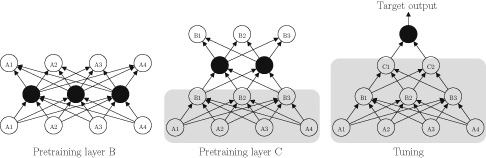
Figure 4.5 The pretraining and tuning stages in greedy layer-wise pretraining. Black circles represent the neurons whose training is the primary objective at each training stage. The gray background marks the components in the network that are frozen during each training stage. Layer-wise pretraining was important in the evolution of deep learning because it was the first approach to training deep networks that was widely adopted.9 However, today most deep learning networks are trained without using layer-wise pretraining. In the mid-2000s, researchers began to appreciate that the vanishing gradient problem was not a strict theoretical limit, but was instead a practical obstacle that could be overcome. The vanishing gradient problem does not cause the error gradients to disappear entirely; there are still gradients being backpropagated through the early layers of the network, it is just that they are very small. Today, there are a number of factors that have been identified as important in successfully training a deep network.
In the mid-2000s, researchers began to appreciate that the vanishing gradient problem was not a strict theoretical limit, but was instead a practical obstacle that could be overcome.
Weight Initialization and ReLU Activation Functions
One factor that is important in successfully training a deep network is how the network weights are initialized. The principles controlling how weight initialization affects the training of a network are still not clear. There are, however, weight initialization procedures that have been empirically shown to help with training a deep network. Glorot initialization10 is a frequently used weight initialization procedure for deep networks. It is based on a number of assumptions but has empirical success to support its use. To get an intuitive understanding of Glorot initialization, consider the fact that there is typically a relationship between the magnitude of values in a set and the variance of the set: generally the larger the values in a set, the larger the variance of the set. So, if the variance calculated on a set of gradients propagated through a layer at one point in the network is similar to the variance for the set of gradients propagated through another layer in a network, it is likely that the magnitude of the gradients propagated through both of these layers will also be similar. Furthermore, the variance of gradients in a layer can be related to the variance of the weights in the layer, so a potential strategy to maintain gradients flowing through a network is to ensure similar variances across each of the layer in a network. Glorot initialization is designed to initialize the weight in a network in such a way that all of the layers in a network will have a similar variance in terms of both forward pass activations and the gradients propagated during the backward pass in backpropagation. Glorot initialization defines a heuristic rule to meet this goal that involves sampling the weights for a network using the following uniform distribution (where w is the weight on a connection between layer j and j+i that is being initialized, U[-a,a] is the uniform distribution over the interval (-a,a),
is the number of neurons in layer
, and the notation w ~ U indicates that the value of w is sampled from distribution U)11:
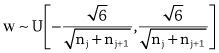
Another factor that contributes to the success or failure of training a deep network is the selection of the activation function used in the neurons. Backpropagating an error gradient through a neuron involves multiplying the gradient by the value of the derivative of the activation function at the activation value of the neuron recorded during the forward pass. The derivatives of the logistic and tanh activation functions have a number of properties that can exacerbate the vanishing gradient problem if they are used in this multiplication step. Figure 4.6 presents a plot of the logistic function and the derivative of the logistic function. The maximum value of the derivative is 0.25. Consequently, after an error gradient has been multiplied by the value of the derivative of the logistic function at the appropriate activation for the neuron, the maximum value the gradient will have is a quarter of the gradient prior to the multiplication. Another problem with using the logistic function is that there are large portions of the domain of the function where the function is saturated (returning values that very close to 0 or 1), and the rate of change of the function in these regions is near zero; thus, the derivative of the function is near 0. This is an undesirable property when backpropagating error gradients because the error gradients will be forced to zero (or close to zero) when backpropagated through any neuron whose activation is within one of these saturated regions. In 2011 it was shown that switching to a rectified linear activation function,
, improved training for deep feedforward neural networks (Glorot et al. 2011). Neurons that use a rectified linear activation function are known as rectified linear units (ReLUs). One advantage of ReLUs is that the activation function is linear for the positive portion of its domain with a derivative equal to 1. This means that gradients can flow easily through ReLUs that have positive activation. However, the drawback of ReLUs is that the gradient of the function for the negative part of its domain is zero, so ReLUs do not train in this portion of the domain. Although undesirable, this is not necessarily a fatal flaw for learning because when backpropagating through a layer of ReLUs the gradients can still flow through the ReLUs in the layers that have positive activation. Furthermore, there are a number of variants of the basic ReLU that introduce a gradient on the negative side of the domain, a commonly used variant being the leaky ReLU (Maas et al. 2013). Today, ReLUs (or variants of ReLUs) are the most frequently used neurons in deep learning research.
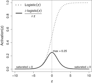
Figure 4.6 Plots of the logistic function and the derivative of the logistic function. The Virtuous Cycle: Better Algorithms, Faster Hardware, Bigger Data
Although improved weight initialization methods and new activation functions have both contributed to the growth of deep learning, in recent years the two most important factors driving deep learning have been the speedup in computer power and the massive increase in dataset sizes. From a computational perspective, a major breakthrough for deep learning occurred in the late 2000s with the adoption of graphical processing units (GPUs) by the deep learning community to speed up training. A neural network can be understood as a sequence of matrix multiplications that are interspersed with the application of nonlinear activation functions, and GPUs are optimized for very fast matrix multiplication. Consequently, GPUs are ideal hardware to speed up neural network training, and their use has made a significant contribution to the development of the field. In 2004, Oh and Jung reported a twentyfold performance increase using a GPU implementation of a neural network (Oh and Jung 2004), and the following year two further papers were published that demonstrated the potential of GPUs to speed up the training of neural networks: Steinkraus et al. (2005) used GPUs to train a two-layer neural network, and Chellapilla et al. (2006) used GPUs to train a CNN. However, at that time there were significant programming challenges to using GPUs for training networks (the training algorithm had to be implemented as a sequence of graphics operations), and so the initial adoption of GPUs by neural network researchers was relatively slow. These programming challenges were significantly reduced in 2007 when NVIDIA (a GPU manufacturer) released a C-like programming interface for GPUs called CUDA (compute unified device architecture).12 CUDA was specifically designed to facilitate the use of GPUs for general computing tasks. In the years following the release of CUDA, the use of GPUs to speed up neural network training became standard.
However, even with these more powerful computer processors, deep learning would not have been possible unless massive datasets had also become available. The development of the internet and social media platforms, the proliferation of smartphones and “internet of things” sensors, has meant that the amount of data being captured has grown at an incredible rate over the last ten years. This has made it much easier for organizations to gather large datasets. This growth in data has been incredibly important to deep learning because neural network models scale well with larger data (and in fact they can struggle with smaller datasets). It has also prompted organizations to consider how this data can be used to drive the development of new applications and innovations. This in turn has driven a need for new (more complex) computational models in order to deliver these new applications. And, the combination of large data and more complex algorithms requires faster hardware in order to make the necessary computational workload tractable. Figure 4.7 illustrates the virtuous cycle between big data, algorithmic breakthroughs (e.g., better weight initialization, ReLUs, etc.), and improved hardware that is driving the deep learning revolution.
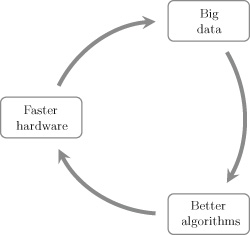
Figure 4.7 The virtuous cycle driving deep learning. Figure inspired by figure 1.2 in Reagen et al. 2017. Summary
The history of deep learning reveals a number of underlying themes. There has been a shift from simple binary inputs to more complex continuous valued input. This trend toward more complex inputs is set to continue because deep learning models are most useful in high-dimensional domains, such as image processing and language. Images often have thousands of pixels in them, and language processing requires the ability represents and process hundreds of thousands of different words. This is why some of the best-known applications of deep learning are in these domains, for example, Facebook’s face-recognition software, and Google’s neural machine translation system. However, there are a growing number of new domains where large and complex digital datasets are being gathered. One area where deep learning has the potential to make a significant impact within the coming years is healthcare, and another complex domain is the sensor rich field of self-driving cars.
Somewhat surprisingly, at the core of these powerful models are simple information processing units: neurons. The connectionist idea that useful complex behavior can emerge from the interactions between large numbers of simple processing units is still valid today. This emergent behavior arises through the sequences of layers in a network learning a hierarchical abstraction of increasingly complex features. This hierarchical abstraction is achieved by each neuron learning a simple transformation of the input it receives. The network as a whole then composes these sequences of smaller transformations in order to apply a complex (highly) nonlinear mapping to the input. The output from the model is then generated by the final output layers of neuron, based the learned representation generated through the hierarchical abstraction. This is why depth is such an important factor in neural networks: the deeper the network, the more powerful the model becomes in terms of its ability to learn complex nonlinear mappings. In many domains, the relationship between input data and desired outputs involves just such complex nonlinear mappings, and it is in these domains that deep learning models outdo other machine learning approaches.
An important design choice in creating a neural network is deciding which activation function to use within the neurons in a network. The activation function within each neuron in a network is how nonlinearity is introduced into the network, and as a result it is a necessary component if the network is to learn a nonlinear mapping from inputs to output. As networks have evolved, so too have the activation functions used in them. New activation functions have emerged throughout the history of deep learning, often driven by the need for functions with better properties for error-gradient propagation: a major factor in the shift from threshold to logistic and tanh activation functions was the need for differentiable functions in order to apply backpropagation; the more recent shift to ReLUs was, similarly, driven by the need to improve the flow of error gradients through the network. Research on activations functions is ongoing, and new functions will be developed and adopted in the coming years.
Another important design choice in creating a neural network is to decide on the structure of the network: for example, how should the neurons in the network be connected together? In the next chapter, we will discuss two very different answers to this question: convolution neural networks and recurrent neural networks.
5 Convolutional and Recurrent Neural Networks
Tailoring the structure of a network to the specific characteristics of the data from a task domain can reduce the training time of the network, and improves the accuracy of the network. Tailoring can be done in a number of ways, such as: constraining the connections between neurons in adjacent layers to subsets (rather than having fully connected layers); forcing neurons to share weights; or introducing backward connections into the network. Tailoring in these ways can be understood as building domain knowledge into the network. Another, related, perspective is it helps the network to learn by constraining the set of possible functions that it can learn, and by so doing guides the network to find a useful solution. It is not always clear how to fit a network structure to a domain, but for some domains where the data has a very regular structure (e.g., sequential data such as text, or gridlike data such as images) there are well-known network architectures that have proved successful. This chapter will introduce two of the most popular deep learning architectures: convolutional neural networks and recurrent neural networks.
Convolutional Neural Networks
Convolution neural networks (CNNs) were designed for image recognition tasks and were originally applied to the challenge of handwritten digit recognition (Fukushima 1980; LeCun 1989). The basic design goal of CNNs was to create a network where the neurons in the early layer of the network would extract local visual features, and neurons in later layers would combine these features to form higher-order features. A local visual feature is a feature whose extent is limited to a small patch, a set of neighboring pixels, in an image. For example, when applied to the task of face recognition, the neurons in the early layers of a CNN learn to activate in response to simple local features (such as lines at a particular angle, or segments of curves), neurons deeper in the network combine these low-level features into features that represent body parts (such as eyes or noises), and the neurons in the final layers of the network combine body part activations in order to be able to identify whole faces in an image.
Using this approach, the fundamental task in image recognition is learning the feature detection functions that can robustly identify the presence, or absence, of local visual features in an image. The process of learning functions is at the core of neural networks, and is achieved by learning the appropriate set of weights for the connections in the network. CNNs learn the feature detection functions for local visual features in this way. However, a related challenge is designing the architecture of the network so that the network will identify the presence of a local visual feature in an image irrespective of where in the image it occurs. In other words, the feature detection functions must be able to work in a translation invariant manner. For example, a face recognition system should be able to recognize the shape of an eye in an image whether the eye is in the center of the image or in the top-right corner of the image. This need for translation invariance has been a primary design principle of CNNs for image processing, as Yann LeCun stated in 1989:
It seems useful to have a set of feature detectors that can detect a particular instance of a feature anywhere on the input plane. Since the precise location of a feature is not relevant to the classification, we can afford to lose some position information in the process. (LeCun 1989, p. 14)CNNs achieve this translation invariance of local visual feature detection by using weight sharing between neurons. In an image recognition setting, the function implemented by a neuron can be understood as a visual feature detector. For example, neurons in the first hidden layer of the network will receive a set of pixel values as input and output a high activation if a particular pattern (local visual feature) is present in this set of pixels. The fact that the function implemented by a neuron is defined by the weights the neuron uses means that if two neurons use the same set of weights then they both implement the same function (feature detector). In chapter 4, we introduced the concept of a receptive field to describe the area that a neuron receives its input from. If two neurons share the same weights but have different receptive fields (i.e., each neuron inspects different areas of the input), then together the neurons act as a feature detector that activates if the feature occurs in either of the receptive fields. Consequently, it is possible to design a network with translation invariant feature detection by creating a set of neurons that share the same weights and that are organized so that: (1) each neuron inspects a different portion of the image; and (2) together the receptive fields of the neurons cover the entire image.
The scenario of searching an image in a dark room with a flashlight that has a narrow beam is sometimes used to explain how a CNN searches an image for local features. At each moment you can point the flashlight at a region of the image and inspect that local region. In this flashlight metaphor, the area of the image illuminated by the flashlight at any moment is equivalent to the receptive field of a single neuron, and so pointing the flashlight at a location is equivalent to applying the feature detection function to that local region. If, however, you want to be sure you inspect the whole image, then you might decide to be more systematic in how you direct the flashlight. For example, you might begin by pointing the flashlight at the top-left corner of the image and inspecting that region. You then move the flashlight to the right, across the image, inspecting each new location as it becomes visible, until you reach the right side of the image. You then point the flashlight back to the left of the image, but just below where you began, and move across the image again. You repeat this process until you reach the bottom-right corner of the image. The process of sequentially searching across an image and at each location in the search applying the same function to the local (illuminated) region is the essence of convolving a function across an image. Within a CNN, this sequential search across an image is implemented using a set of neurons that share weights and whose union of receptive fields covers the entire image.
Figure 5.1 illustrates the different stages of processing that are often found in a CNN. The
matrix on the left of the figure represents the image that is the input to the CNN. The
matrix immediately to the right of the input represents a layer of neurons that together search the entire image for the presence of a particular local feature. Each neuron in this layer is connected to a different
receptive field (area) in the image, and they all apply the same weight matrix to their inputs:
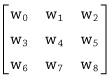
The receptive field of the neuron
(top-left) in this layer is marked with the gray square covering the
area in the top-left of the input image. The dotted arrows emerging from each of the locations in this gray area represent the inputs to neuron
. The receptive field of the neighboring neuron
is indicated by
square, outlined in bold in the input image. Notice that the receptive fields of these two neurons overlap. The amount of overlap of receptive fields is controlled by a hyperparameter called the stride length. In this instance, the stride length is one, meaning that for each position moved in the layer the receptive field of the neuron is translated by the same amount on the input. If the stride length hyperparameter is increased, the amount of overlap between receptive fields is decreased.
The receptive fields of both of these neurons (
and
) are matrices of pixel values and the weights used by these neurons are also matrices. In computer vision, the matrix of weights applied to an input is known as the kernel (or convolution mask); the operation of sequentially passing a kernel across an image and within each local region, weighting each input and adding the result to its local neighbors, is known as a convolution. Notice that a convolution operation does not include a nonlinear activation function (this is applied at a later stage in processing). The kernel defines the feature detection function that all the neurons in the convolution implement. Convolving a kernel across an image is equivalent to passing a local visual feature detector across the image and recording all the locations in the image where the visual feature was present. The output from this process is a map of all the locations in the image where the relevant visual feature occurred. For this reason, the output of a convolution process is sometimes known as a feature map. As noted above, the convolution operation does not include a nonlinear activation function (it only involves a weighted summation of the inputs). Consequently, it is standard to apply a nonlinearity operation to a feature map. Frequently, this is done by applying a rectified linear function to each position in a feature map; the rectified linear activation function is defined as:
. Passing a rectified linear activation function over a feature map simply changes all negative values to 0. In figure 5.1, the process of updating a feature map by applying a rectified linear activation function to each of its elements is represented by the layer labeled Nonlinearity.
The quote from Yann LeCun, at the start of this section, mentions that the precise location of a feature in an image may not be relevant to an image processing task. With this in mind, CNNs often discard location information in favor of generalizing the network’s ability to do image classification. Typically, this is achieved by down-sampling the updated feature map using a pooling layer. In some ways pooling is similar to the convolution operation described above, in so far as pooling involves repeatedly applying the same function across an input space. For pooling, the input space is frequently a feature map whose elements have been updated using a rectified linear function. Furthermore, each pooling operation has a receptive field on the input space—although, for pooling, the receptive fields sometimes do not overlap. There are a number of different pooling functions used; the most common is called max pooling, which returns the maximum value of any of its inputs. Calculating the average value of the inputs is also used as a pooling function.
Convolving a kernel across an image is equivalent to passing a local visual feature detector across the image and recording all the locations in the image where the visual feature was present.
The operation sequence of applying a convolution, followed by a nonlinearity, to the feature map, and then down-sampling using pooling, is relatively standard across most CNNs. Often these three operations are together considered to define a convolutional layer in a network, and this is how they are presented in figure 5.1.
The fact that a convolution searches an entire image means that if the visual feature (pixel pattern) that the function (defined by shared kernel) detects occurs anywhere in the image, its presence will be recorded in the feature map (and if pooling is used, also in the subsequent output from the pooling layer). In this way, a CNN supports translation invariant visual feature detection. However, this has the limitation that the convolution can only identify a single type of feature. CNNs generalize beyond one feature by training multiple convolutional layers in parallel (or filters), with each filter learning a single kernel matrix (feature detection function). Note the convolution layer in figure 5.1 illustrates a single filter. The outputs of multiple filters can be integrated in a variety of ways. One way to integrate information from different filters is to take the feature maps generated by the separate filters and combine them into a single multifilter feature map. A subsequent convolutional layer then takes this multifilter feature map as input. Another other way to integrate information from different filter is to use a densely connected layer of neurons. The final layer in figure 5.1 illustrates a dense layer. This dense layer operates in exactly the same way as a standard layer in a fully connected feedforward network. Each neuron in the dense layer is connected to all of the elements output by each of the filters, and each neuron learns a set of weights unique to itself that it applies to the inputs. This means that each neuron in a dense layer can learn a different way to integrate information from across the different filters.
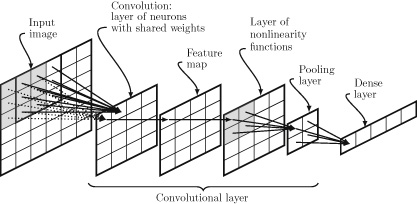
Figure 5.1 Illustrations of the different stages of processing in a convolutional layer. Note in this figure the Image and Feature Map are data structures; the other stages represent operations on data. The AlexNet CNN, which won the ImageNet Large-Scale Visual Recognition Challenge (ILSVRC) in 2012, had five convolutional layers, followed by three dense layers. The first convolutional layer had ninety-six different kernels (or filters) and included a ReLU nonlinearity and pooling. The second convolution layer had 256 kernels and also included ReLU nonlinearity and pooling. The third, fourth, and fifth convolutional layers did not include a nonlinearity step or pooling, and had 384, 384, and 256 kernels, respectively. Following the fifth convolutional layer, the network had three dense layers with 4096 neurons each. In total, AlexNet had sixty million weights and 650,000 neurons. Although sixty million weights is a large number, the fact that many of the neurons shared weights actually reduced the number of weights in the network. This reduction in the number of required weights is one of the advantages of CNN networks. In 2015, Microsoft Research developed a CNN network called ResNet, which won the ILSVRC 2015 challenge (He et al. 2016). The ResNet architecture extended the standard CNN architecture using skip-connections. A skip-connection takes the output from one layer in the network and feeds it directly into a layer that may be much deeper in the network. Using skip-connections it is possible to train very deep networks. In fact, the ResNet model developed by Microsoft Research had a depth of 152 layers.
Recurrent Neural Networks
Recurrent neural networks (RNNs) are tailored to the processing of sequential data. An RNN processes a sequence of data by processing each element in the sequence one at time. An RNN network only has a single hidden layer, but it also has a memory buffer that stores the output of this hidden layer for one input and feeds it back into the hidden layer along with the next input from the sequence. This recurrent flow of information means that the network processes each input within the context generated by processing the previous input, which in turn was processed in the context of the input preceding it. In this way, the information that flows through the recurrent loop encodes contextual information from (potentially) all of the preceding inputs in the sequence. This allows the network to maintain a memory of what it has seen previously in the sequence to help it decide what to do with the current input. The depth of an RNN arises from the fact that the memory vector is propagated forward and evolved through each input in the sequence; as a result an RNN network is considered as deep as a sequence is long.
The depth of an RNN arises from the fact that the memory vector is propagated forward and evolved through each input in the sequence; as a result an RNN network is considered as deep as a sequence is long.
Figure 5.2 illustrates the architecture of an RNN and shows how information flows through the network as it processes a sequence. At each time step, the network in this figure receives a vector containing two elements as input. The schematic on the left of figure 5.2 (time step=1.0) shows the flow of information in the network when it receives the first input in the sequence. This input vector is fed forward into the three neurons in the hidden layer of the network. At the same time these neurons also receive whatever information is stored in the memory buffer. Because this is the initial input, the memory buffer will only contain default initialization values. Each of the neurons in the hidden layer will process the input and generate an activation. The schematic in the middle of figure 5.2 (time step=1.5) shows how this activation flows on through the network: the activation of each neuron is passed to the output layer where it is processed to generate the output of the network, and it is also stored in the memory buffer (overwriting whatever information was stored there). The elements of the memory buffer simply store the information written to them; they do not transform it in any way. As a result, there are no weights on the edges going from the hidden units to the buffer. There are, however, weights on all the other edges in the network, including those from the memory buffer units to the neurons in the hidden layer. At time step 2, the network receives the next input from the sequence, and this is passed to the hidden layer neurons along with the information stored in the buffer. This time the buffer contains the activations that were generated by the hidden neurons in response to the first input.
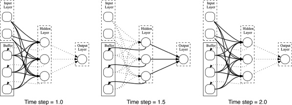
Figure 5.2 The flow of information in an RNN as it processes a sequence of inputs. The arrows in bold are the active paths of information flow at each time point; the dashed arrows show connections that are not active at that time. Figure 5.3 shows an RNN that has been unrolled through time as it processes a sequence of inputs
. Each box in this figure represents a layer of neurons. The box labeled
represents the state of the memory buffer when the network is initialized; the boxes labeled
represent the hidden layer of the network at each time step; and the boxes labeled
represent the output layer of the network at each time step. Each of the arrows in the figure represents a set of connections between one layer and another layer. For example, the vertical arrow from
to
represents the connections between the input layer and the hidden layer at time step 1. Similarly, the horizontal arrows connecting the hidden layers represent the storing of the activations from a hidden state at one time step in the memory buffer (not shown) and the propagation of these activations to the hidden layer at the next time step through the connections from the memory buffer to the hidden state. At each time step, an input from the sequence is presented to the network and is fed forward to the hidden layer. The hidden layer generates a vector of activations that is passed to the output layer and is also propagated forward to the next time step along the horizontal arrows connecting the hidden states.
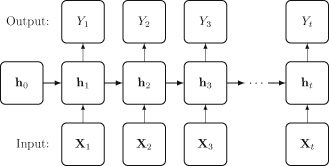
Figure 5.3 An RNN network unrolled through time as it processes a sequence of inputs [x1,x2,……,xt] Although RNNs can process a sequence of inputs, they struggle with the problem of vanishing gradients. This is because training an RNN to process a sequence of inputs requires the error to be backpropagated through the entire length of the sequence. For example, for the network in figure 5.3, the error calculated on the output
must be backpropagated through the entire network so that it can be used to update the weights on the connections from
and
to
. This entails backpropagating the error through all the hidden layers, which in turn involves repeatedly multiplying the error by the weights on the connections feeding activations from one hidden layer forward to the next hidden layer. A particular problem with this process is that it is the same set of weights that are used on all the connections between the hidden layers: each horizontal arrow represents the same set of connections between the memory buffer and the hidden layer, and the weights on these connections are stationary through time (i.e., they don’t change from one time step to the next during the processing of a given sequence of inputs). Consequently, backpropogating an error through k time steps involves (among other multiplications) multiplying the error gradient by the same set of weights k times. This is equivalent to multiplying each error gradient by a weight raised to the power of k. If this weight is less than 1, then when it is raised to a power, it diminishes at an exponential rate, and consequently, the error gradient also tends to diminish at an exponential rate with respect to the length of the sequence—and vanish.
Long short-term memory networks (LSTMs) are designed to reduce the effect of vanishing gradients by removing the repeated multiplication by the same weight vector during backpropagation in an RNN. At the core of an LSTM1 unit is a component called the cell. The cell is where the activation (the short-term memory) is stored and propagated forward. In fact, the cell often maintains a vector of activations. The propagation of the activations within the cell through time is controlled by three components called gates: the forget gate, the input gate, and the output gate. The forget gate is responsible for determining which activations in the cell should be forgotten at each time step, the input gate controls how the activations in the cell should be updated in response to the new input, and the output gate controls what activations should be used to generate the output in response to the current input. Each of the gates consists of layers of standard neurons, with one neuron in the layer per activation in the cell state.
Figure 5.4 illustrates the internal structure of an LSTM cell. Each of the arrows in this image represents a vector of activations. The cell runs along the top of the figure from left (
) to right (
). Activations in the cell can take values in the range -1 to +1. Stepping through the processing for a single input, the input vector
is first concatenated with the hidden state vector that has been propagated forward from the preceding time step
. Working from left to right through the processing of the gates, the forget gate takes the concatenation of the input and the hidden state and passes this vector through a layer of neurons that use a sigmoid (also known as logistic)2 activation function. As a result of the neurons in the forget layer using sigmoid activation functions the output of this forget layer is a vector of values in the range 0 to 1. The cell state is then multiplied by this forget vector. The result of this multiplication is that activations in the cell state that are multiplied by components in the forget vector with values near 0 are forgotten, and activations that are multiplied by forget vector components with values near 1 are remembered. In effect, multiplying the cell state by the output of a sigmoid layer acts as a filter on the cell state.
Next, the input gate decides what information should be added to the cell state. The processing in this step is done by the components in the middle block of figure 5.4, marked Input. This processing is broken down into two subparts. First, the gate decides which elements in the cell state should be updated, and second it decides what information should be included in the update. The decision regarding which elements in the cell state should be updated is implemented using a similar filter mechanism to the forget gate: the concatenated input
plus hidden state
is passed through a layer of sigmoid units to generate a vector of elements, the same width as the cell, where each element in the vector is in the range 0 to 1; values near 0 indicate that the corresponding cell element will not be updated, and values near 1 indicate that the corresponding cell element will be updated. At the same time that the filter vector is generated, the concatenated input and hidden state are also passed through a layer of tanh units (i.e., neurons that use the tanh activation function). Again, there is one tanh unit for each activation in the LSTM cell. This vector represents the information that may be added to the cell state. Tanh units are used to generate this update vector because tanh units output values in the range -1 to +1, and consequently the value of the activations in the cell elements can be both increased and decreased by an update.3 Once these two vectors have been generated, the final update vector is calculated by multiplying the vector output from the tanh layer by the filter vector generated from the sigmoid layer. The resulting vector is then added to the cell using vector addition.
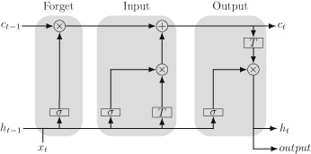
Figure 5.4 Schematic of the internal structure of an LSTM unit: σ represents a layer of neurons with sigmoid activations, T represents a layer of neurons with tanh activations, × represents vector multiplication, and + represents vector addition. The figure is inspired by an image by Christopher Olah available at: http://colah.github.io/posts/2015-08-Understanding-LSTMs/. The final stage of processing in an LSTM is to decide which elements of the cell should be output in response to the current input. This processing is done by the components in the block marked Output (on the right of figure 5.4). A candidate output vector is generated by passing the cell through a tanh layer. At the same time, the concatenated input and propagated hidden state vector are passed through a layer of sigmoid units to create another filter vector. The actual output vector is then calculated by multiplying the candidate output vector by this filter vector. The resulting vector is then passed to the output layer, and is also propagated forward to the next time step as the new hidden state
.
The fact that an LSTM unit contains multiple layers of neurons means that an LSTM is a network in itself. However, an RNN can be constructed by treating an LSTM as the hidden layer in the RNN. In this configuration, an LSTM unit receives an input at each time step and generates an output for each input. RNNs that use LSTM units are often known as LSTM networks.
LSTM networks are ideally suited for natural language processing (NLP). A key challenge in using a neural network to do natural language processing is that the words in language must be converted into vectors of numbers. The word2vec models, created by Tomas Mikolov and colleagues at Google research, are one of the most popular ways of doing this conversion (Mikolov et al. 2013). The word2vec models are based on the idea that words that appear in similar contexts have similar meanings. The definition of context here is surrounding words. So for example, the words London and Paris are semantically similar because each of them often co-occur with words that the other word also co-occurs with, such as: capital, city, Europe, holiday, airport, and so on. The word2vec models are neural networks that implement this idea of semantic similarity by initially assigning random vectors to each word and then using co-occurrences within a corpus to iteratively update these vectors so that semantically similar words end up with similar vectors. These vectors (known as word embeddings) are then used to represent a word when it is being input to a neural network.
One of the areas of NLP where deep learning has had a major impact is in machine translation. Figure 5.5 presents a high-level schematic of the seq2seq (or encoder-decoder) architecture for neural machine translation (Sutskever et al. 2014). This architecture is composed of two LSTM networks that have been joined together. The first LSTM network processes the input sentence in a word-by-word fashion. In this example, the source language is French. The words are entered into the system in reverse order as it has been found that this leads to better translations. The symbol
is a special end of sentence symbol. As each word is entered, the encoder updates the hidden state and propagates it forward to the next time step. The hidden state generated by the encoder in response to the
symbol is taken to be a vector representation of the input sentence. This vector is passed as the initial input to the decoder LSTM. The decoder is trained to output the translation sentence word by word, and after each word has been generated, this word is fed back into the system as the input for the next time step. In a way, the decoder is hallucinating the translation because it uses its own output to drive its own generation process. This process continues until the decoder outputs an

symbol.
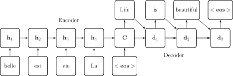
Figure 5.5 Schematic of the seq2seq (or encoder-decoder) architecture. The idea of using a vector of numbers to represent the (interlingual) meaning of a sentence is very powerful, and this concept has been extended to the idea of using vectors to represent intermodal/multimodal representations. For example, an exciting development in recent years has been the development of automatic image captioning systems. These systems can take an image as input and generate a natural language description of the image. The basic structure of these systems is very similar to the neural machine translation architecture shown in figure 5.5. The main difference is that the encoder LSTM network is replaced by a CNN architecture that processes the input image and generates a vector representation that is then propagated to the decoder LSTM (Xu et al. 2015). This is another example of the power of deep learning arising from its ability to learn complex representations of information. In this instance, the system learns intermodal representations that enable information to flow from what is in an image to language. Combining CNN and RNN architectures is becoming more and more popular because it offers the potential to integrate the advantages of both systems and enables deep learning architectures to handle very complex data.
Irrespective of the network architecture we use, we need to find the correct weights for the network if we wish to create an accurate model. The weights of a neuron determine the transformation the neuron applies to its inputs. So, it is the weights of the network that define the fundamental building blocks of the representation the network learns. Today the standard method for finding these weights is an algorithm that came to prominence in the 1980s: backpropagation. The next chapter will present a comprehensive introduction to this algorithm.
6 Learning Functions
A neural network model, no matter how deep or complex, implements a function, a mapping from inputs to outputs. The function implemented by a network is determined by the weights the network uses. So, training a network (learning the function the network should implement) on data involves searching for the set of weights that best enable the network to model the patterns in the data. The most commonly used algorithm for learning patterns from data is the gradient descent algorithm. The gradient descent algorithm is very like the perceptron learning rule and the LMS algorithm described in chapter 4: it defines a rule to update the weights used in a function based on the error of the function. By itself the gradient descent algorithm can be used to train a single output neuron. However, it cannot be used to train a deep network with multiple hidden layers. This limitation is because of the credit assignment problem: how should the blame for the overall error of a network be shared out among the different neurons (including the hidden neurons) in the network? Consequently, training a deep neural network involves using both the gradient descent algorithm and the backpropagation algorithm in tandem.
The process used to train a deep neural network can be characterized as: randomly initializing the weight of a network, and then iteratively updating the weights of the network, in response to the errors the network makes on a dataset, until the network is working as expected. Within this training framework, the backpropagation algorithm solves the credit (or blame) assignment problem, and the gradient descent algorithm defines the learning rule that actually updates the weights in the network.
This chapter is the most mathematical chapter in the book. However, at a high level, all you need to know about the backpropagation algorithm and the gradient descent algorithm is that they can be used to train deep networks. So, if you don’t have the time to work through the details in this chapter, feel free to skim through it. If, however, you wish to get a deeper understanding of these two algorithms, then I encourage you to engage with the material. These algorithms are at the core of deep learning and understanding how they work is, possibly, the most direct way of understanding its potentials and limitations. I have attempted to present the material in this chapter in an accessible way, so if you are looking for a relatively gentle but still comprehensive introduction to these algorithms, then I believe that this will provide it for you. The chapter begins by explaining the gradient descent algorithm, and then explains how gradient descent can be used in conjunction with the backpropagation algorithm to train a neural network.
Gradient Descent
A very simple type of function is a linear mapping from a single input to a single output. Table 6.1 presents a dataset with a single input feature and a single output. Figure 6.1 presents a scatterplot of this data along with a plot of the line that best fits this data. This line can be used as a function to map from an input value to a prediction of the output value. For example, if x = 0.9, then the response returned by this linear function is y = 0.6746. The error (or loss) of using this line as a model for the data is shown by the dashed lines from the line to each datum.
Table 6.1. A sample dataset with one input feature, x, and an output (target) feature, y
X Y 0.72 0.54 0.45 0.56 0.23 0.38 0.76 0.57 0.14 0.17 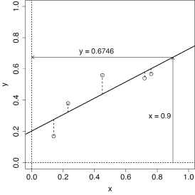
Figure 6.1 Scatterplot of data with “best fit” line and the errors of the line on each example plotted as vertical dashed line segments. The figure also shows the mapping defined by the line for input x=0.9 to output y=0.6746. In chapter 2, we described how a linear function can be represented using the equation of a line:

where
is the slope of the line, and
is the y-intercept, which specifies where the line crosses the y-axis. For the line in figure 6.1,
and
; this is why the function returns the value
when
, as in the following:
The slope
and the y-intercept
are the parameters of this model, and these parameters can be varied to fit the model to the data.
The equation of a line has a close relationship with the weighted sum operation used in a neuron. This becomes apparent if we rewrite the equation of a line with model parameters rewritten as weights (
:
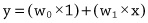
Different lines (different linear models for the data) can be created by varying either of these weights (or model parameters). Figure 6.2 illustrates how a line changes as the intercept and slope of the line varies: the dashed line illustrates what happens if the y-intercept is increased, and the dotted line shows what happens if the slope is decreased. Changing the y-intercept
vertically translates the line, whereas modifying the slope
rotates the line around the point
.
Each of these new lines defines a different function, mapping from
to
, and each function will have a different error with respect to how well it matches the data. Looking at figure 6.2, we can see that the full line,
, fits the data better than the other two lines because on average it passes closer to the data points. In other words, on average the error for this line for each data point is less than those of the other two lines. The total error of a model on a dataset can be measured by summing together the error the model makes on each example in the dataset. The standard way to calculate this total error is to use an equation known as the sum of squared errors (SSE):
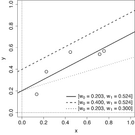
Figure 6.2 Plot illustrating how a line changes as the intercept (w0) and slope (w1) are varied. 
This equation tells us how to add together the errors of a model on a dataset containing n examples. This equation calculates for each of the
examples in the dataset the error of the model by subtracting the prediction of the target value returned by the model from the correct target value for that example, as specified in the dataset. In this equation
is the correct output value for target feature listed in the dataset for example j, and
is the estimate of the target value returned by the model for the same example. Each of these errors is then squared and these squared errors are then summed. Squaring the errors ensures that they are all positive, and therefore in the summation the errors for examples where the function underestimated the target do not cancel out the errors on examples where it overestimated the target. The multiplication of the summation of the errors by
, although not important for the current discussion, will become useful later. The lower the SSE of a function, the better the function models the data. Consequently, the sum of squared errors can be used as a fitness function to evaluate how well a candidate function (in this situation a model instantiating a line) matches the data.
Figure 6.3 shows how the error of a linear model varies as the parameters of the model change. These plots show the SSE of a linear model on the example single-input–single-output dataset listed in table 6.1. For each parameter there is a single best setting and as the parameter moves away from this setting (in either direction) the error of the model increases. A consequence of this is that the error profile of the model as each parameter varies is convex (bowl-shaped). This convex shape is particularly apparent in the top and middle plots in figure 6.3, which show that the SSE of the model is minimized when
(lowest point of the curve in the top plot), and when
(lowest point of the curve in the middle plot).
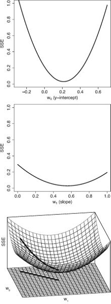
Figure 6.3 Plots of the changes in the error (SSE) of a linear model as the parameters of the model change. Top: the SSE profile of a linear model with a fixed slope w1=0.524 when w0 ranges across the interval 0.3 to 1. Middle: the SSE profile of a linear model with a y-intercept fixed at w0=0.203 when w1 ranges across the interval 0 to 1. Bottom: the error surface of the linear model when both w0 and w1 are varied. If we plot the error of the model as both parameters are varied, we generate a three-dimensional convex bowl-shaped surface, known as an error surface. The bowl-shaped mesh in the plot at the bottom of figure 6.3 illustrates this error surface. This error surface was created by first defining a weight space. This weight space is represented by the flat grid at the bottom of the plot. Each coordinate in this weight space defines a different line because each coordinate specifies an intercept (a
value) and slope (a
value). Consequently, moving across this planar weight space is equivalent to moving between different models. The second step in constructing the error surface is to associate an elevation with each line (i.e., coordinate) in the weight space. The elevation associated with each weight space coordinate is the SSE of the model defined by that coordinate; or, put more directly, the height of the error surface above the weight space plane is the SSE of the corresponding linear model when it is used as a model for the dataset. The weight space coordinates that correspond with the lowest point of the error surface define the linear model that has the lowest SSE on the dataset (i.e., the linear model that best fits the data).
The shape of the error surface in the plot on the right of figure 6.3 indicates that there is only a single best linear model for this dataset because there is a single point at the bottom of the bowl that has a lower elevation (lower error) than any other points on the surface. Moving away from this best model (by varying the weights of the model) necessarily involves moving to a model with a higher SSE. Such a move is equivalent to moving to a new coordinate in the weight space, which has a higher elevation associated with it on the error surface. A convex or bowl-shaped error surface is incredibly useful for learning a linear function to model a dataset because it means that the learning process can be framed as a search for the lowest point on the error surface. The standard algorithm used to find this lowest point is known as gradient descent.
A convex or bowl-shaped error surface is incredibly useful for learning a linear function to model a dataset because it means that the learning process can be framed as a search for the lowest point on the error surface.
The gradient descent algorithm begins by creating an initial model using a randomly selected a set of weights. Next the SSE of this randomly initialized model is calculated. Taken together, the guessed set of weights and the SSE of the corresponding model define the initial starting point on the error surface for the search. It is very likely that the randomly initialized model will be a bad model, so it is very likely that the search will begin at a location that has a high elevation on the error surface. This bad start, however, is not a problem, because once the search process is positioned on the error surface, the process can find a better set of weights by simply following the gradient of the error surface downhill until it reaches the bottom of the error surface (the location where moving in any direction results in an increase in SSE). This is why the algorithm is known as gradient descent: the gradient that the algorithm descends is the gradient of the error surface of the model with respect to the data.
An important point is that the search does not progress from the starting location to the valley floor in one weight update. Instead, it moves toward the bottom of the error surface in an iterative manner, and during each iteration the current set of weights are updated so as to move to a nearby location in the weight space that has a lower SSE. Reaching the bottom of the error surface can take a large number of iterations. An intuitive way of understanding the process is to imagine a hiker who is caught on the side of a hill when a thick fog descends. Their car is parked at the bottom of the valley; however, due to the fog they can only see a few feet in any direction. Assuming that the valley has a nice convex shape to it, they can still find their way to their car, despite the fog, by repeatedly taking small steps that move down the hill following the local gradient at the position they are currently located. A single run of a gradient descent search is illustrated in the bottom plot of figure 6.3. The black curve plotted on the error surface illustrates the path the search followed down the surface, and the black line on the weight space plots the corresponding weight updates that occurred during the journey down the error surface. Technically, the gradient descent algorithm is known as an optimization algorithm because the goal of the algorithm is to find the optimal set of weights.
The most important component of the gradient descent algorithm is the rule that defines how the weights are updated during each iteration of the algorithm. In order to understand how this rule is defined it is first necessary to understand that the error surface is made up of multiple error gradients. For our simple example, the error surface is created by combining two error curves. One error curve is defined by the changes in the SSE as
changes, shown in the top plot of figure 6.3. The other error curve is defined by the changes in the SSE as
changes, shown in the plot in the middle of figure 6.3. Notice that the gradient of each of these curves can vary along the curve, for example, the
error curve has a steep gradient on the extreme left and right of the plot, but the gradient becomes somewhat shallower in the middle of the curve. Also, the gradients of two different curves can vary dramatically; in this particular example the
error curve generally has a much steeper gradient than the
error curve.
The fact that the error surface is composed of multiple curves, each with a different gradient, is important because the gradient descent algorithm moves down the combined error surface by independently updating each weight so as to move down the error curve associated with that weight. In other words, during a single iteration of the gradient descent algorithm,
is updated to move down the
error curve and
is updated the move down the
error curve. Furthermore, the amount each weight is updated in an iteration is proportional to the steepness of the gradient of the weight’s error curve, and this gradient will vary from one iteration to the next as the process moves down the error curve. For example,
will be updated by relatively large amounts in iterations where the search process is located high up on either side of the
error curve, but by smaller amounts in iterations where the search process is nearer to the bottom of the
error curve.
The error curve associated with each weight is defined by how the SSE changes with respect to the change in the value of the weight. Calculus, and in particular differentiation, is the field of mathematics that deals with rates of change. For example, taking the derivative of a function,
, calculates the rate of change of
(the output) for each unit change in
(the input). Furthermore, if a function takes multiple inputs [
] then it is possible to calculate the rate of change of the output,
, with respect to changes in each of these inputs,
, by taking the partial derivative of the function of with respect to each input. The partial derivative of a function with respect to a particular input is calculated by first assuming that all the other inputs are held constant (and so their rate of change is 0 and they disappear from the calculation) and then taking the derivative of what remains. Finally, the rate of change of a function for a given input is also known as the gradient of the function at the location on the curve (defined by the function) that is specified by the input. Consequently, the partial derivative of the SSE with respect to a weight specifies how the output of the SSE changes as that weight changes, and so it specifies the gradient of the error curve of the weight. This is exactly what is needed to define the gradient descent weight update rule: the partial derivative of the SSE with respect to a weight specifies how to calculate the gradient of the weight’s error curve, and in turn this gradient specifies how the weight should be updated to reduce the error (the output of the SSE).
The partial derivative of a function with respect to a particular variable is the derivative of the function when all the other variables are held constant. As a result there is a different partial derivative of a function with respect to each variable, because a different set of terms are considered constant in the calculation of each of the partial derivatives. Therefore, there is a different partial derivative of the SSE for each weight, although they all have a similar form. This is why each of the weights is updated independently in the gradient descent algorithm: the weight update rule is dependent on the partial derivative of the SSE for each weight, and because there is a different partial derivative for each weight, there is a separate weight update rule for each weight. Again, although the partial derivative for each weight is distinct, all of these derivatives have the same form, and so the weight update rule for each weight will also have the same form. This simplifies the definition of the gradient descent algorithm. Another simplifying factor is that the SSE is defined relative to a dataset with
examples. The relevance of this is that the only variables in the SSE are the weights; the target output
and the inputs
are all specified by the dataset for each example, and so can be considered constants. As a result, when calculating the partial derivative of the SSE with respect to a weight, many of the terms in the equation that do not include the weight can be deleted because they are considered constants.
The relationship between the output of the SSE and each weight becomes more explicit if the SSE definition is rewritten so that the term
, denoting the output predicted by the model, is replaced by the structure of the model generating the prediction. For the model with a single input
and a dummy input,
this rewritten version of the SSE is:
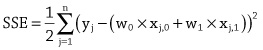
This equation uses a double subscript on the inputs, the first subscript
identifies the example (or row in the dataset) and the second subscript specifies the feature (or column in the dataset) of the input. For example,
represents feature 1 from example
. This definition of the SSE can be generalized to a model with
inputs:
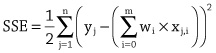
Calculating the partial derivative of the SSE with respect to a specific weight involves the application of the chain rule from calculus and a number of standard differentiation rules. The result of this derivation is the following equation (for simplicity of presentation we switch back to the notation
to represent the output from the model):
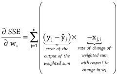
This partial derivative specifies how to calculate the error gradient for weight
for the dataset where
is the input associated with
for each example in the dataset. This calculation involves multiplying two terms, the error of the output and the rate of change of the output (i.e., the weighted sum) with respect to changes in the weight. One way of understanding this calculation is that if changing the weight changes the output of the weighted sum by a large amount, then the gradient of the error with respect to the weight is large (steep) because changing the weight will result in big changes in the error. However, this gradient is the uphill gradient, and we wish to move the weights so as to move down the error curve. So in the gradient descent weight update rule (shown below) the “–” sign in front of the input
is dropped. Using
to represent the iteration of the algorithm (an iteration involves a single pass through the
examples in the dataset), the gradient descent weight update rule is defined as:
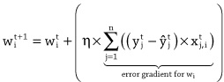
There are a number of notable factors about this weight update rule. First, the rule specifies how the weight
should be updated after iteration
through the dataset. This update is proportional to the gradient of the error curve for the weight for that iteration (i.e., the summation term, which actually defines the partial derivative of the SSE for that weight). Second, the weight update rule can be used to update the weights for functions with multiple inputs. This means that the gradient descent algorithm can be used to descend error surfaces with more than two weight coordinates. It is not possible to visualize these error surfaces because they will have more than three dimensions, but the basic principles of descending an error surface using the error gradient generalizes to learning functions with multiple inputs. Third, although the weight update rule has a similar structure for each weight, the rule does define a different update for each weight during each iteration because the update is dependent on the inputs in the dataset examples to which the weight is applied. Fourth, the summation in the rule indicates that, in each iteration of the gradient descent algorithm, the current model should be applied to all
of the examples in the dataset. This is one of the reasons why training a deep learning network is such a computationally expensive task. Typically for very large datasets, the dataset is split up into batches of examples sampled from the dataset, and each iteration of training is based on a batch, rather than the entire dataset. Fifth, apart from the modifications necessary to include the summation, this rule is identical to the LMS (also known as the Widrow-Hoff or delta) learning rule introduced in chapter 4, and the rule implements the same logic: if the output of the model is too large, then weights associated with positive inputs should be reduced; if the output is too small, then these weights should be increased. Moreover, the purpose and function of the learning rate hyperparameter (η) is the same as in the LMS rule: scale the weight adjustments to ensure that the adjustments aren’t so large that the algorithm misses (or steps over) the best set of weights. Using this weight update rule, the gradient descent algorithm can be summarized as follows:
1. Construct a model using an initial set of weights.
2. Repeat until the model performance is good enough.
a. Apply the current model to the examples in the dataset.
b. Adjust each weight using the weight update rule.
3. Return the final model.One consequence of the independent updating of weights, and the fact that weight updates are proportional to the local gradient on the associated error curve, is that the path the gradient descent algorithm follows to the lowest point on the error surface may not be a straight line. This is because the gradient of each of the component error curves may not be equal at each location on the error surface (the gradient for one of the weights may be steeper than the gradient for the other weight). As a result, one weight may be updated by a larger amount than another weight during a given iteration, and thus the descent to the valley floor may not follow a direct route. Figure 6.4 illustrates this phenomenon. Figure 6.4 presents a set of top-down views of a portion of a contour plot of an error surface. This error surface is a valley that is quite long and narrow with steeper sides and gentler sloping ends; the steepness is reflected by the closeness of the contours. As a result, the search initially moves across the valley before turning toward the center of the valley. The plot on the left illustrates the first iteration of the gradient descent algorithm. The initial starting point is the location where the three arrows, in this plot, meet. The lengths of the dotted and dashed arrows represent the local gradients of the
and
error curves, respectively. The dashed arrow is longer than the dotted arrow reflecting the fact that the local gradient of the
error curve is steeper than that of the
error curve. In each iteration, each of the weights is updated in proportion to the gradient of their error curve; so in the first iteration, the update for
is larger than for
and therefore the overall movement is greater across the valley than along the valley. The thick black arrow illustrates the overall movement in the underlying weight space, resulting from the weight updates in this first iteration. Similarly, the middle plot illustrates the error gradients and overall weight update for the next iteration of gradient descent. The plot on the right shows the complete path of descent taken by the search process from initial location to the global minimum (the lowest point on the error surface).
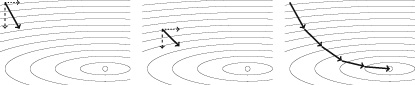
Figure 6.4 Top-down views of a portion of a contour plot of an error surface, illustrating the gradient descent path across the error surface. Each of the thick arrows illustrates the overall movement of the weight vector for a single iteration of the gradient descent algorithm. The length of dotted and dashed arrows represent the local gradient of the w0 and w1 error curves, respectively, for that iteration. The plot on the right shows the overall path taken to the global minimum of the error surface.
It is relatively straightforward to map the weight update rule over to training a single neuron. In this mapping, the weightIt is relatively straightforward to map the weight update rule over to training a single neuron. In this mapping, the weight
is the bias term for a neuron, and the other weights are associated with the other inputs to the neuron. The derivation of the partial derivative of the SSE is dependent on the structure of the function that generates
. The more complex this function is, the more complex the partial derivative becomes. The fact that the function a neuron defines includes both a weighted summation and an activation function means that the partial derivative of the SSE with respect to a weight in a neuron is more complex than the partial derivative given above. The inclusion of the activation function within the neuron results in an extra term in the partial derivative of the SSE. This extra term is the derivative of the activation function with respect to the output from the weighted summation function. The derivative of the activation function is with respect to the output of the weighted summation function because this is the input that the activation function receives. The activation function does not receive the weight directly. Instead, the changes in the weight only affect the output of the activation function indirectly through the effect that these weight changes have on the output of the weighted summation. The main reason why the logistic function was such a popular activation function in neural networks for so long was that it has a very straightforward derivative with respect to its inputs. The gradient descent weight update rule for a neuron using the logistic function is as follows:
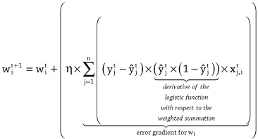
The fact that the weight update rule includes the derivative of the activation function means that the weight update rule will change if the activation function of the neuron is changed. However, this change will simply involve updating the derivative of the activation function; the overall structure of the rule will remain the same.
This extended weight update rule means that the gradient descent algorithm can be used to train a single neuron. It cannot, however, be used to train neural networks with multiple layers of neurons because the definition of the error gradient for a weight depends on the error of the output of the function, the term
. Although it is possible to calculate the error of the output of a neuron in the output layer of the network by directly comparing the output with the expected output, it is not possible to calculate this error term directly for the neurons in the hidden layer of the network, and as a result it is not possible to calculate the error gradients for each weight. The backpropagation algorithm is a solution to the problem of calculating error gradients for the weights in the hidden layers of the network.
Training a Neural Network Using Backpropagation
The term backpropagation has two different meanings. The primary meaning is that it is an algorithm that can be used to calculate, for each neuron in a network, the sensitivity (gradient/rate-of-change) of the error of the network to changes in the weights. Once the error gradient for a weight has been calculated, the weight can then be adjusted to reduce the overall error of the network using a weight update rule similar to the gradient descent weight update rule. In this sense, the backpropagation algorithm is a solution to the credit assignment problem, introduced in chapter 4. The second meaning of backpropagation is that it is a complete algorithm for training a neural network. This second meaning encompasses the first sense, but also includes a learning rule that defines how the error gradients of the weights should be used to update the weights within the network. Consequently, the algorithm described by this second meaning involves a two-step process: solve the credit assignment problem, and then use the error gradients of the weights, calculated during credit assignment, to update the weights in the network. It is useful to distinguish between these two meanings of backpropagation because there are a number of different learning rules that can be used to update the weights, once the credit assignment problem has been resolved. The learning rule that is most commonly used with backpropagation is the gradient descent algorithm introduced earlier. The description of the backpropagation algorithm given here focuses on the first meaning of backpropagation, that of the algorithm being a solution to the credit assignment problem.
Backpropagation: The Two-Stage Algorithm
The backpropagation algorithm begins by initializing all the weights of the network using random values. Note that even a randomly initialized network can still generate an output when an input is presented to the network, although it is likely to be an output with a large error. Once the network weights have been initialized, the network can be trained by iteratively updating the weights so as to reduce the error of the network, where the error of the network is calculated in terms of the difference between the output generated by the network in response to an input pattern, and the expected output for that input, as defined in the training dataset. A crucial step in this iterative weight adjustment process involves solving the credit assignment problem, or, in other words, calculating the error gradients for each weight in the network. The backpropagation algorithm solves this problem using a two-stage process. In first stage, known as the forward pass, an input pattern is presented to the network, and the resulting neuron activations flow forward through the network until an output is generated. Figure 6.5 illustrates the forward pass of the backpropagation algorithm. In this figure, the weighted summation of inputs calculated at each neuron (e.g.,
represents the weighted summation of inputs calculated for neuron 1) and the outputs (or activations, e.g.,
represents the activation for neuron 1) of each neuron is shown. The reason for listing the
and
values for each neuron in this figure is to highlight the fact that during the forward pass both of these values, for each neuron, are stored in memory. The reason they are stored in memory is that they are used in the backward pass of the algorithm. The
value for a neuron is used to calculate the update to the weights on input connections to the neuron. The
value for a neuron is used to calculate the update to the weights on the output connections from a neuron. The specifics of how these values are used in the backward pass will be described below.
The second stage, known as the backward pass, begins by calculating an error gradient for each neuron in the output layer. These error gradients represent the sensitivity of the network error to changes in the weighted summation calculation of the neuron, and they are often denoted by the shorthand notation
(pronounced delta) with a subscript indicating the neuron. For example, δk is the gradient of the network error with respect to small changes in the weighted summation calculation of the neuron k. It is important to recognize that there are two different error gradients calculated in the backpropagation algorithm:
1. The first is thevalue for each neuron. The
for each neuron is the rate of change of the error of the network with respect to changes in the weighted summation calculation of the neuron. There is one
for each neuron. It is these
error gradients that the algorithm backpropagates.
2. The second is the error gradient of the network with respect to changes in the weights of the network. There is one of these error gradients for each weight in the network. These are the error gradients that are used to update the weights in the network. However, it is necessary to first calculate theterm for each neuron (using backpropagation) in order to calculate the error gradients for the weights.
Note there is only a single
per neuron, but there may be many weights associated with that neuron, so the
term for a neuron may be used in the calculation of multiple weight error gradients.
Once the
s for the output neurons have been calculated, the
s for the neurons in the last hidden layer are then calculated. This is done by assigning a portion of the
from each output neuron to each hidden neuron that is directly connected to it. This assignment of blame, from output neuron to hidden neuron, is dependent on the weight of the connection between the neurons, and the activation of the hidden neuron during the forward pass (this is why the activations are recorded in memory during the forward pass). Once the blame assignment, from the output layer, has been completed, the
for each neuron in the last hidden layer is calculated by summing the portions of the
s assigned to the neuron from all of the output neurons it connects to. The same process of blame assignment and summing is then repeated to propagate the error gradient back from the last layer of hidden neurons to the neurons in the second last layer, and so on, back to the input layer. It is this backward propagation of
s through the network that gives the algorithm its name. At the end of this backward pass there is a
calculated for each neuron in the network (i.e., the credit assignment problem has been solved) and these
s can then be used to update the weights in the network (using, for example, the gradient descent algorithm introduced earlier). Figure 6.6 illustrates the backward pass of the backpropagation algorithm. In this figure, the
s get smaller and smaller as the backpropagation process gets further from the output layer. This reflects the vanishing gradient problem discussed in chapter 4 that slows down the learning rate of the early layers of the network.

Figure 6.5 The forward pass of the backpropagation algorithm. In summary, the main steps within each iteration of the backpropagation algorithm are as follows:
1. Present an input to the network and allow the neuron activations to flow forward through the network until an output is generated. Record both the weighted sum and the activation of each neuron.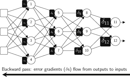
Figure 6.6 The backward pass of the backpropagation algorithm. 2. Calculate a
(delta) error gradient for each neuron in the output layer.
3. Backpropagate theerror gradients to obtain a
(delta) error gradient for each neuron in the network.
4. Use theerror gradients and a weight update algorithm, such as gradient descent, to calculate the error gradients for the weights and use these to update the weights in the network.
The algorithm continues iterating through these steps until the error of the network is reduced (or converged) to an acceptable level.
Backpropagation: Backpropagating the δ s
A
term of a neuron describes the error gradient for the network with respect to changes in the weighted summation of inputs calculated by the neuron. To help make this more concrete, figure 6.7 (top) breaks open the processing stages within a neuron
and uses the term
to denote the result of the weighted summation within the neuron. The neuron in this figure receives inputs (or activations) from three other neurons (
), and
is the weighted sum of these activations. The output of the neuron,
, is then calculated by passing
through a nonlinear activation function,
, such as the logistic function. Using this notation a
for a neuron
is the rate of change of the error of the network with respect to small changes in the value of
. Mathematically, this term is the partial derivative of the networks error with respect to
:

No matter where in a network a neuron is located (output layer or hidden layer), the
for the neuron is calculated as the product of two terms:
1. the rate of change of the network error in response to changes in the neuron’s activation (output):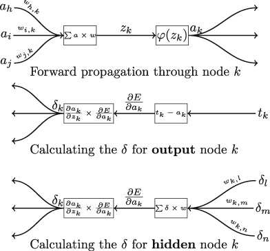
Figure 6.7 Top: the forward propagation of activations through the weighted sum and activation function of a neuron. Middle: The calculation of the δ term for an output neuron (tk is the expected activation for the neuron and ak is the actual activation). Bottom: The calculation of the δ term for a hidden neuron. This figure is loosely inspired by figure 5.2 and figure 5.3 in Reed and Marks II 1999. 2. the rate of change of the activation of the neuron with respect to changes in the weighted sum of inputs to the neuron:
.
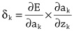
Figure 6.7 (middle) illustrates how this product is calculated for neurons in the output layer of a network. The first step is to calculate the rate of change of the error of the network with respect to the output of the neuron, the term
. Intuitively, the larger the difference between the activation of a neuron,
, and the expected activation,
, the faster the error can be changed by changing the activation of the neuron. So the rate of change of the error of the network with respect to changes in the activation of an output neuron
can be calculated by subtracting the neuron’s activation (
) from the expected activation (
):

This term connects the error of the network to the output of the neuron. The neuron’s
, however, is the rate of change of the error with respect to the input to the activation function (
), not the output of that function (
). Consequently, in order to calculate the
for the neuron, the
value must be propagated back through the activation function to connect it to the input to the activation function. This is done by multiplying
by the rate of change of the activation function with respect to the input value to the function,
. In figure 6.7, the rate of change of the activation function with respect to its input is denoted by the term:
. This term is calculated by plugging the value
(stored from the forward pass through the network) into the equation of the derivative of the activation function with respect to
. For example, the derivative of the logistic function with respect to its input is:

Figure 6.8 plots this function and shows that plugging a
value into this equation will result in a value between 0 and 0.25. For example, figure 6.8 shows that if
then
. This is why the weighted summation value for each neuron (
) is stored during the forward pass of the algorithm.
The fact1 that the calculation of a neuron’s
involves a product that includes the derivative of the neuron’s activation function makes it necessary to be able to take the derivative of the neuron’s activation function. It is not possible to take the derivative of a threshold activation function because there is a discontinuity in the function at the threshold. As a result, the backpropagation algorithm does not work for networks composed of neurons that use threshold activation functions. This is one of the reasons why neural networks moved away from threshold activation and started to use the logistic and tanh activation functions. The logistic and tanh functions both have very simple derivatives and this made them particularly suitable to backpropagation.

Figure 6.8 Plots of the logistic function and the derivative of the logistic function. Figure 6.7 (bottom) illustrates how the
for a neuron in a hidden layer is calculated. This involves the same product of terms as was used for neurons in the output layer. The difference is that the calculation of the
is more complex for hidden units. For hidden neurons, it is not possible to directly connect the output of the neuron with the error of a network. The output of a hidden neuron only indirectly affects the overall error of the network through the variations that it causes in the downstream neurons that receive the output as input, and the magnitude of these variations is dependent on the weight each of these downstream neurons applies to the output. Furthermore, this indirect effect on the network error is in turn dependent on the sensitivity of the network error to these later neurons, that is, their
values. Consequently, the sensitivity of the network error to the output of a hidden neuron can be calculated as a weighted sum of the
values of the neurons immediately downstream of the neuron:
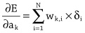
As a result, the error terms (the
values) for all the downstream neurons to which a neuron’s output is passed in the forward pass must be calculated before the
for neuron k can be calculated. This, however, is not a problem because in the backward pass the algorithm is working backward through the network and will have calculated the
terms for the downstream neurons before it reaches neuron k.
For hidden neurons, the other term in the
product,
, is calculated in the same way as it is calculated for output neurons: the
value for the neuron (the weighted summation of inputs, stored during the forward pass through the network) is plugged into the derivative of the neuron’s activation function with respect to
.
Backpropagation: Updating the Weights
The fundamental principle of the backpropagation algorithm in adjusting the weights in a network is that each weight in a network should be updated in proportion to the sensitivity of the overall error of the network to changes in that weight. The intuition is that if the overall error of the network is not affected by a change in a weight, then the error of the network is independent of that weight, and, therefore, the weight did not contribute to the error. The sensitivity of the network error to a change in an individual weight is measured in terms of the rate of change of the network error in response to changes in that weight.
The fundamental principle of the backpropagation algorithm in adjusting the weights in a network is that each weight in a network should be updated in proportion to the sensitivity of the overall error of the network to changes in that weight.
The overall error of a network is a function with multiple inputs: both the inputs to the network and all the weights in the network. So, the rate of change of the error of a network in response to changes in a given network weight is calculated by taking the partial derivative of the network error with respect to that weight. In the backpropagation algorithm, the partial derivative of the network error for a given weight is calculated using the chain rule. Using the chain rule, the partial derivative of the network error with respect a weight
on the connection between a neuron
and a neuron
is calculated as the product of two terms:
1. the first term describes the rate of change of the weighted sum of inputs in neuronwith respect to changes in the weight
;
2. and the second term describes the rate of change of the network error in response to changes in the weighted sum of inputs calculated by the neuron. (This second term is the
for neuron
.)
Figure 6.9 shows how the product of these two terms connects a weight to the output error of the network. The figure shows the processing of the last two neurons (
and
) in a network with a single path of activation. Neuron
receives a single input
and the output from neuron
is the sole input to neuron
. The output of neuron
is the output of the network. There are two weights in this portion of the network,
and
.
The calculations shown in figure 6.9 appear complicated because they contain a number of different components. However, as we will see, by stepping through these calculations, each of the individual elements is actually easy to calculate; it’s just keeping track of all the different elements that poses a difficulty.
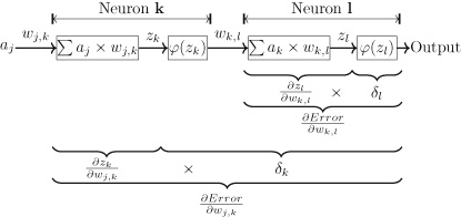
Figure 6.9 An illustration of how the product of derivatives connects weights in the network to the error of the network. Focusing on
, this weight is applied to an input of the output neuron of the network. There are two stages of processing between this weight and the network output (and error): the first is the weighted sum calculated in neuron
; the second is the nonlinear function applied to this weighted sum by the activation function of neuron
. Working backward from the output, the
term is calculated using the calculation shown in the middle figure of figure 6.7: the difference between the target activation for the neuron and the actual activation is calculated and is multiplied by the partial derivative of the neuron’s activation function with respect to its input (the weighted sum
),
. Assuming that the activation function used by neuron
is the logistic function, the term
is calculated by plugging in the value
(stored during the forward pass of the algorithm) into the derivation of the logistic function:
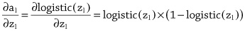
So the calculation of
under the assumption that neuron
uses a logistic function is:

The
term connects the error of the network to the input to the activation function (the weighted sum
). However, we wish to connect the error of the network back to the weight
. This is done by multiplying the
term by the partial derivative of the weighted summation function with respect to weight
:
. This partial derivative describes how the output of the weighted sum function
changes as the weight
changes. The fact that the weighted summation function is a linear function of weights and activations means that in the partial derivative with respect to a particular weight all the terms in the function that do not involve the specific weight go to zero (are considered constants) and the partial derivative simplifies to just the input associated with that weight, in this instance input
.

This is why the activations for each neuron in the network are stored in the forward pass. Taken together these two terms,
and
, connect the weight
to the network error by first connecting the weight to
, and then connecting
to the activation of the neuron, and thereby to the network error. So, the error gradient of the network with respect to changes in weight
is calculated as:

The other weight in the figure 6.9 network,
, is deeper in the network, and, consequently, there are more processing steps between it and the network output (and error). The
term for neuron
is calculated, through backpropagation (as shown at the bottom of figure 6.7), using the following product of terms:
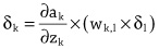
Assuming the activation function used by neuron
is the logistic function, then the term
is calculated in a similar way to
: the value
is plugged into the equation for the derivative of the logistic function. So, written out in long form the calculation of
is:

However, in order to connect the weight
with the error of the network, the term
must be multiplied by the partial derivative of the weighted summation function with respect to the weight:
. As described above, the partial derivative of a weighted sum function with respect to a weight reduces to the input associated with the weight
(i.e.,
); and the gradient of the networks error with respect to the hidden weight
is calculated by multiplying
by
Consequently, the product of the terms (
and
) forms a chain connecting the weight
to the network error. For completeness, the product of terms for
, assuming logistic activation functions in the neurons, is:
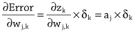
Although this discussion has been framed in the context of a very simple network with only a single path of connections, it generalizes to more complex networks because the calculation of the
terms for hidden units already considers the multiple connections emanating from a neuron. Once the gradient of the network error with respect to a weight has been calculated (
), the weight can be adjusted so as to reduce the weight of the network using the gradient descent weight update rule. Here is the weight update rule, specified using the notation from backpropagation, for the weight on the connection between neuron
and neuron
during iteration
of the algorithm:

Finally, an important caveat on training neural networks with backpropagation and gradient descent is that the error surface of a neural network is much more complex than that of a linear models. Figure 6.3 illustrated the error surface of a linear model as a smooth convex bowl with a single global minimum (a single best set of weights). However, the error surface of a neural network is more like a mountain range with multiple valleys and peaks. This is because each of the neurons in a network includes a nonlinear function in its mapping of inputs to outputs, and so the function implemented by the network is a nonlinear function. Including a nonlinearity within the neurons of a network increases the expressive power of the network in terms of its ability to learn more complex functions. However, the price paid for this is that the error surface becomes more complex and the gradient descent algorithm is no longer guaranteed to find the set of weights that define the global minimum on the error surface; instead it may get stuck within a minima (local minimum). Fortunately, however, backpropagation and gradient descent can still often find sets of weights that define useful models, although searching for useful models may require running the training process multiple times to explore different parts of the error surface landscape.
7 The Future of Deep Learning
On March 27, 2019, Yoshua Bengio, Geoffrey Hinton, and Yann LeCun jointly received the ACM A.M. Turing award. The award recognized the contributions they have made to deep learning becoming the key technology driving the modern artificial intelligence revolution. Often described as the “Nobel Prize for Computing,” the ACM A.M Turing award carries a $1 million prize. Sometimes working together, and at other times working independently or in collaboration with others, these three researchers have, over a number of decades of work, made numerous contributions to deep learning, ranging from the popularization of backpropagation in the 1980s, to the development of convolutional neural networks, word embeddings, attention mechanisms in networks, and generative adversarial networks (to list just some examples). The announcement of the award noted the astonishing recent breakthroughs that deep learning has led to in computer vision, robotics, speech recognition, and natural language processing, as well as the profound impact that these technologies are having on society, with billions of people now using deep learning based artificial intelligence on a daily basis through smart phones applications. The announcement also highlighted how deep learning has provided scientists with powerful new tools that are resulting in scientific breakthroughs in areas as diverse as medicine and astronomy. The awarding of this prize to these researchers reflects the importance of deep learning to modern science and society. The transformative effects of deep learning on technology is set to increase over the coming decades with the development and adoption of deep learning continuing to be driven by the virtuous cycle of ever larger datasets, the development of new algorithms, and improved hardware. These trends are not stopping, and how the deep learning community responds to them will drive growth and innovations within the field over the coming years.
Big Data Driving Algorithmic Innovations
Chapter 1 introduced the different types of machine learning: supervised, unsupervised, and reinforcement learning. Most of this book has focused on supervised learning, primarily because it is the most popular form of machine learning. However, a difficulty with supervised learning is that it can cost a lot of money and time to annotate the dataset with the necessary target labels. As datasets continue to grow, the data annotation cost is becoming a barrier to the development of new applications. The ImageNet dataset1 provides a useful example of the scale of the annotation task involved in deep learning projects. This data was released in 2010, and is the basis for the ImageNet Large-Scale Visual Recognition Challenge (ILSVRC). This is the challenge that the AlexNet CNN won in 2012 and the ResNet system won in 2015. As was discussed in chapter 4, AlexNet winning the 2012 ILSVRC challenge generated a lot of excitement about deep learning models. However, the AlexNet win would not have been possible without the creation of the ImageNet dataset. This dataset contains more than fourteen million images that have been manually annotated to indicate which objects are present in each image; and more than one million of the images have actually been annotated with the bounding boxes of the objects in the image. Annotating data at this scale required a significant research effort and budget, and was achieved using crowdsourcing platforms. It is not feasible to create annotated datasets of this size for every application.
As datasets continue to grow, the data annotation cost is becoming a barrier to the development of new applications.
One response to this annotation challenge has been a growing interest in unsupervised learning. The autoencoder models used in Hinton’s pretraining (see chapter 4) are one neural network approach to unsupervised learning, and in recent years different types of autoencoders have been proposed. Another approach to this problem is to train generative models. Generative models attempt to learn the distribution of the data (or, to model the process that generated the data). Similar to autoencoders, generative models are often used to learn a useful representation of the data prior to training a supervised model. Generative adversarial networks (GANs) are an approach to training generative models that has received a lot of attention in recent years (Goodfellow et al. 2014). A GAN consists of two neural networks, a generative model and a discriminative model, and a sample of real data. The models are trained in an adversarial manner. The task of the discriminative model is to learn to discriminate between real data sampled from the dataset, and fake data that has been synthesized by the generator. The task of the generator is to learn to synthesize fake data that can fool the discriminative model. Generative models trained using a GAN can learn to synthesize fake images that mimic an artistic style (Elgammal et al. 2017), and also to synthesize medical images along with lesion annotations (Frid-Adar et al. 2018). Learning to synthesize medical images, along with the segmentation of the lesions in the synthesized image, opens the possibility of automatically generating massive labeled datasets that can be used for supervised learning. A more worrying application of GANs is the use of these networks to generate deep fakes: a deep fake is a fake video of a person doing something they never did that is created by swapping their face into a video of someone else. Deep fakes are very hard to detect, and have been used maliciously on a number of occasions to embarrass public figures, or to spread fake news stories.
Another solution to the data labeling bottleneck is that rather than training a new model from scratch for each new application, we rather repurpose models that have been trained on a similar task. Transfer learning is the machine learning challenge of using information (or representations) learned on one task to aid learning on another task. For transfer learning to work, the two tasks should be from related domains. Image processing is an example of a domain where transfer learning is often used to speed up the training of models across different tasks. Transfer learning is appropriate for image processing tasks because low-level visual features, such as edges, are relatively stable and useful across nearly all visual categories. Furthermore, the fact that CNN models learn a hierarchy of visual feature, with the early layers in CNN learning functions that detect these low-level visual features in the input, makes it possible to repurpose the early layers of pretrained CNNs across multiple image processing projects. For example, imagine a scenario where a project requires an image classification model that can identify objects from specialized categories for which there are no samples in general image datasets, such as ImageNet. Rather than training a new CNN model from scratch, it is now relatively standard to first download a state-of-the-art model (such as the Microsoft ResNet model) that has been trained on ImageNet, then replace the later layers of the model with a new set of layers, and finally to train this new hybrid-model on a relatively small dataset that has been labeled with the appropriate categories for the project. The later layers of the state-of-the-art (general) model are replaced because these layers contain the functions that combine the low-level features into the task specific categories the model was originally trained to identify. The fact that the early layers of the model have already been trained to identify the low-level visual features speeds up the training and reduces the amount of data needed to train the new project specific model.
The increased interest in unsupervised learning, generative models, and transfer learning can all be understood as a response to the challenge of annotating increasingly large datasets.
The Emergence of New Models
The rate of emergence of new deep learning models is accelerating every year. A recent example is capsule networks (Hinton et al. 2018; Sabour et al. 2017). Capsule networks are designed to address some of the limitations of CNNs. One problem with CNNs, sometimes known as the Picasso problem, is the fact that a CNN ignores the precise spatial relationships between high-level components within an object’s structure. What this means in practice is that a CNN that has been trained to identify faces may learn to identify the shapes of eyes, the nose, and the mouth, but will not learn the required spatial relationships between these parts. Consequently, the network can be fooled by an image that contains these body parts, even if they are not in the correct relative position to each other. This problem arises because of the pooling layers in CNNs that discard positional information.
At the core of capsule networks is the intuition that the human brain learns to identify object types in a viewpoint invariant manner. Essentially, for each object type there is an object class that has a number of instantiation parameters. The object class encodes information such as the relative relationship of different object parts to each other. The instantiation parameters control how the abstract description of an object type can be mapped to the specific instance of the object that is currently in view (for example, its pose, scale, etc.).
A capsule is a set of neurons that learns to identify whether a specific type of object or object part is present at a particular location in an image. A capsule outputs an activity vector that represents the instantiation parameters of the object instance, if one is present at the relevant location. Capsules are embedded within convolutional layers. However, capsule networks replace the pooling process, which often defines the interface between convolutional layers, with a process called dynamic routing. The idea behind dynamic routing is that each capsule in one layer in the network learns to predict which capsule in the next layer is the most relevant capsule for it to forward its output vector to.
At the time or writing, capsule networks have the state-of-the-art performance on the MNIST handwritten digit recognition dataset that the original CNNs were trained on. However, by today’s standards, this is a relatively small dataset, and capsule networks have not been scaled to larger datasets. This is partly because the dynamic routing process slows down the training of capsule networks. However, if capsule networks are successfully scaled, then they may introduce an important new form of model that extends the ability of neural networks to analyze images in a manner much closer to the way humans do.
Another recent model that has garnered a lot of interest is the transformer model (Vaswani et al. 2017). The transformer model is an example of a growing trend in deep learning where models are designed to have sophisticated internal attention mechanisms that enable a model to dynamically select subsets of the input to focus on when generating an output. The transformer model has achieved state-of-the-art performance on machine translation for some language pairs, and in the future this architecture may replace the encoder-decoder architecture described in chapter 5. The BERT (Bidirectional Encoder Representations from Transformers) model has built on the Transformer architecture (Devlin et al. 2018). The BERT development is particularly interesting because at its core is the idea of transfer learning (as discussed above in relation to the data annotation bottleneck). The basic approach to creating a natural language processing model with BERT is to pretrain a model for a given language using a large unlabeled dataset (the fact that the dataset is unlabeled means that it is relatively cheap to create). This pretrained model can then be used as the basis to create a models for specific tasks for the language (such as sentiment classification or question answering) by fine-tuning the pretrained model using supervised learning and a relatively small annotated dataset. The success of BERT has shown this approach to be tractable and effective in developing state-of-the-art natural language processing systems.
New Forms of Hardware
Today’s deep learning is powered by graphics processing units (GPUs): specialized hardware that is optimized to do fast matrix multiplications. The adoption, in the late 2000s, of commodity GPUs to speed up neural network training was a key factor in many of the breakthroughs that built momentum behind deep learning. In the last ten years, hardware manufacturers have recognized the importance of the deep learning market and have developed and released hardware specifically designed for deep learning, and which supports deep learning libraries, such as TensorFlow and PyTorch. As datasets and networks continue to grow in size, the demand for faster hardware continues. At the same time, however, there is a growing recognition of the energy costs associated with deep learning, and people are beginning to look for hardware solutions that have a reduced energy footprint.
Neuromorphic computing emerged in the late 1980s from the work of Carver Mead.2 A neuromorphic chip is composed of a very-large-scale integrated (VLSI) circuit, connecting potentially millions of low-power units known as spiking neurons. Compared with the artificial neurons used in standard deep learning systems, the design of a spiking neuron is closer to the behavior of biological neurons. In particular, a spiking neuron does not fire in response to the set of input activations propagated to it at a particular time point. Instead, a spiking neuron maintains an internal state (or activation potential) that changes through time as it receives activation pulses. The activation potential increases when new activations are received, and decays through time in the absence of incoming activations. The neuron fires when its activation potential surpasses a specific threshold. Due to the temporal decay of the neuron’s activation potential, a spiking neuron only fires if it receives the requisite number of input activations within a time window (a spiking pattern). One advantage of this temporal based processing is that spiking neurons do not fire on every propagation cycle, and this reduces the amount of energy the network consumes.
In comparison with traditional CPU design, neuromorphic chips have a number of distinctive characteristics, including:
1. Basic building blocks: traditional CPUs are built using transistor based logic gates (e.g., AND, OR, NAND gates), whereas neuromorphic chips are built using spiking neurons.
2. Neuromorphic chips have an analog aspect to them: in a traditional digital computer, information is sent in high-low electrical bursts in sync with a central clock; in a neuromorphic chip, information is sent as patterns of high-low signals that vary through time.
3. Architecture: the architecture of traditional CPUs is based on the von Neumann architecture, which is intrinsically centralized with all the information passing through the CPU. A neuromorphic chip is designed to allow massive parallelism of information flow between the spiking neurons. Spiking neurons communicate directly with each other rather than via a central information processing hub.
4. Information representation is distributed through time: the information signals propagated through a neuromorphic chip use a distributed representation, similar to the distributed representations discussed in chapter 4, with the distinction that in a neuromorphic chip these representations are also distributed through time. Distributed representations are more robust to information loss than local representations, and this is a useful property when passing information between hundreds of thousands, or millions, of components, some of which are likely to fail.Currently there are a number of major research projects focused on neuromorphic computing. For example, in 2013 the European Commission allocated one billion euros in funding to the ten-year Human Brain Project.3 This project directly employs more than five hundred scientists, and involves research from more than a hundred research centers across Europe. One of the projects key objectives is the development of neuromorphic computing platforms capable of running a simulation of a complete human brain. A number of commercial neuromorphic chips have also been developed. In 2014, IBM launched the TrueNorth chip, which contained just over a million neurons that are connected together by over 286 million synapses. This chip uses approximately 1/10,000th the power of a conventional microprocessor. In 2018, Intel Labs announced the Loihi (pronounced low-ee-hee) neuromorphic chip. The Loihi chip has 131,072 neurons connected together by 130,000,000 synapses. Neuromorphic computing has the potential to revolutionize deep learning; however, it still faces a number of challenges, not least of which is the challenge of developing the algorithms and software patterns for programming this scale of massively parallel hardware.
Finally, on a slightly longer time horizon, quantum computing is another stream of hardware research that has the potential to revolutionize deep learning. Quantum computing chips are already in existence; for example, Intel has created a 49-qubit quantum test chip, code named Tangle Lake. A qubit is the quantum equivalent of a binary digit (bit) in traditional computing. A qubit can store more than one bit of information; however, it is estimated that it will require a system with one million or more qubits before quantum computing will be useful for commercial purposes. The current time estimate for scaling quantum chips to this level is around seven years.
The Challenge of Interpretability
Machine learning, and deep learning, are fundamentally about making data-driven decisions. Although deep learning provides a powerful set of algorithms and techniques to train models that can compete (and in some cases outperform) humans on a range of decision-making tasks, there are many situations where a decision by itself is not sufficient. Frequently, it is necessary to provide not only a decision but also the reasoning behind a decision. This is particularly true when the decision affects a person, be it a medical diagnosis or a credit assessment. This concern is reflected in privacy and ethics regulations in relation to the use of personal data and algorithmic decision-making pertaining to individuals. For example, Recital 714 of the General Data Protection Regulations (GDPR) states that individuals, affected by a decision made by an automated decision-making process, have the right to an explanation with regards to how the decision was reached.
Different machine learning models provide different levels of interpretability with regard to how they reach a specific decision. Deep learning models, however, are possibly the least interpretable. At one level of description, a deep learning model is quite simple: it is composed of simple processing units (neurons) that are connected together into a network. However, the scale of the networks (in terms of the number of neurons and the connections between them), the distributed nature of the representations, and the successive transformations of the input data as the information flows deeper into the network, makes it incredibly difficult to interpret, understand, and therefore explain, how the network is using an input to make a decision.
The legal status of the right to explanation within GDPR is currently vague, and the specific implications of it for machine learning and deep learning will need to be worked out in the courts. This example does, however, highlight the societal need for a better understanding of how deep learning models use data. The ability to interpret and understand the inner workings of a deep learning model is also important from a technical perspective. For example, understanding how a model uses data can reveal if a model has an unwanted bias in how it makes its decisions, and also reveal the corner cases that the model will fail on. The deep learning and the broader artificial intelligence research communities are already responding to this challenge. Currently, there are a number of projects and conferences focused on topics such as explainable artificial intelligence, and human interpretability in machine learning.
Chis Olah and his colleagues summarize the main techniques currently used to examine the inner workings of deep learning models as: feature visualization, attribution, and dimensionality reduction (Olah et al. 2018). One way to understand how a network processes information is to understand what inputs trigger particular behaviors in a network, such as a neuron firing. Understanding the specific inputs that trigger the activation of a neuron enables us to understand what the neuron has learned to detect in the input. The goal of feature visualization is to generate and visualize inputs that cause a specific activity within a network. It turns out that optimization techniques, such a backpropogation, can be used to generate these inputs. The process starts with a random generated input and the input is then iteratively updated until the target behavior is triggered. Once the required necessary input has been isolated, it can then be visualized in order to provide a better understanding of what the network is detecting in the input when it responds in a particular way. Attribution focuses on explaining the relationship between neurons, for example, how the output of a neuron in one layer of the network contributes to the overall output of the network. This can be done by generating a saliency (or heat-map) for the neurons in a network that captures how much weight the network puts on the output of a neuron when making a particular decision. Finally, much of the activity within a deep learning network is based on the processing of high-dimensional vectors. Visualizing data enables us to use our powerful visual cortex to interpret the data and the relationships within the data. However, it is very difficult to visualize data that has a dimensionality greater than three. Consequently, visualization techniques that are able to systematically reduce the dimensionality of high-dimensional data and visualize the results are incredibly useful tools for interpreting the flow of information within a deep network. t-SNE5 is a well-known technique that visualizes high-dimensional data by projecting each datapoint into a two- or three-dimensional map (van der Maaten and Hinton 2008). Research on interpreting deep learning networks is still in its infancy, but in the coming years, for both societal and technical reasons, this research is likely to become a more central concern to the broader deep learning community.
Final Thoughts
Deep learning is ideally suited for applications involving large datasets of high-dimensional data. Consequently, deep learning is likely to make a significant contribution to some of the major scientific challenges of our age. In the last two decades, breakthroughs in biological sequencing technology have made it possible to generate high-precision DNA sequences. This genetic data has the potential to be the foundation for the next generation of personalized precision medicine. At the same time, international research projects, such as the Large Hadron Collider and Earth orbit telescopes, generate huge amounts of data on a daily basis. Analyzing this data can help us to understand the physics of our universe at the smallest and the biggest scales. In response to this flood of data, scientists are, in ever increasing numbers, turning to machine learning and deep learning to enable them to analyze this data.
One way to understand how a network processes information is to understand what inputs trigger particular behaviors in a network, such as a neuron firing.
At a more mundane level, however, deep learning already directly affects our lives. It is likely, that for the last few years, you have unknowingly been using deep learning models on a daily basis. A deep learning model is probably being invoked every time you use an internet search engine, a machine translation system, a face recognition system on your camera or social media website, or use a speech interface to a smart device. What is potentially more worrying is that the trail of data and metadata that you leave as you move through the online world is also being processed and analzsed using deep learning models. This is why it is so important to understand what deep learning is, how it works, what is it capable of, and its current limitations.
-
万里:农村改革从反对“学大寨”开始
本文系作者1997年10月10日,与中共中央党史研究室负责人和记者的谈话的节选
回想一下改革以前,要什么没什么,只能凭证凭票供应,什么粮票、布票,这个票那个票的,连买块肥皂也要票。至于水果,什么香蕉、橘子呀,见也见不到。什么都缺,人们把这种状况叫短缺经济。现在完全变了,短缺变为充足,甚至变为饱和。什么票证也不要了,只要一个票,就是人民币。有了人民币,什么都可以买得到。按总量计算,我们不少农产品名列前茅,甚至世界第一,但一看“人均”就成了后列。这是大国的好处,也是大国的难处。要保证这么一大家子人有饭吃,而且要逐渐逐渐地吃得稍为好一点,是很不容易的。包产到户提高了农民的积极性,使农产品丰富了,这对保证物价稳定,进而保证社会稳定、政治稳定,是个根本性的因素。因此,从人民公社到包产到户不是个小变化,而是个大变化,体制的变化,时代的变化。
过去“左”了那么多年,几乎把农民的积极性打击完了。现在要翻过来,搞包产到户,把农民的积极性再提起来,提得比过去更高,这当然不可能那么容易,要有一个历史过程。我认为这个历史过程,是同“左”倾错误斗争的过程,应当把纠正“左”倾错误作为主线来考虑。
大寨本来是个好典型,特别是自力更生、艰苦奋斗的精神,应当认真学习,发扬光大。但是,“文化大革命”时期,毛主席号召全国学大寨,要树这面红旗,事情就走到反面去了。中国这么大,农村的条件千差万别,只学一个典型,只念大寨“一本经”,这本身就不科学,就不实事求是。何况这时学大寨,并不是学它如何搞农业生产,搞山区建设,而主要是学它如何把阶级斗争的弦绷紧,如何“大批促大干”。大寨也自我膨胀,以为自己事事正确,把“左”倾错误恶性发展到登峰造极的地步,成为“四人帮”推行极“左”路线的工具。
我为什么会有这样看法呢?并不是因为我对大寨有什么成见,而是我到安徽工作以后,从农村的实际中逐渐体会到的。
1977年6月,党中央派我到安徽去当第一书记。我又不熟悉农村工作,所以一到任就先下去看农业、看农民,用三四个月的时间把全省大部分地区都跑到了。我这个长期在城市工作的干部,虽然不能说对农村的贫困毫无所闻,但是到农村一具体接触,还是非常受刺激。原来农民的生活水平这么低啊,吃不饱,穿不暖,住的房子不像个房子的样子。淮北、皖东有些穷村,门、窗都是泥土坯的,连桌子、凳子也是泥土坯的,找不到一件木器家具,真是家徒四壁呀。我真没料到,解放几十年了,不少农村还这么穷!我不能不问自己,这是什么原因?这能算是社会主义吗?人民公社到底有什么问题?当然,人民公社是上了宪法的,我也不能乱说,但我心里已经认定,看来从安徽的实际情况出发,最重要的是怎么调动农民的积极性,否则连肚子也吃不饱,一切无从谈起。
我刚到安徽那一年,全省二十八万多个生产队,只有10%的生产队能维持温饱;67%的队人均年收入低于60元,40元以下的约占25%。我这个第一书记心里怎么能不犯愁啊?越看越听越问心情越沉重,越认定非另找出路不可。于是,回省便找新调来的顾卓新、赵守一反复交换意见,共同研究解决办法。同时,决定派农委的周曰礼他们再去做专题调查,起草对策。随即搞出了一份《关于目前农村经济政策几个问题的规定》(简称“省委六条”),常委讨论通过后,再下去征求意见修改。经过几上几下,拿出了一个正式“草案”。“六条”强调农村一切工作要以生产为中心。我们当时的决心是,不管上面那些假、大、空的叫喊,一定要从安徽的实际情况出发,切切实实解决面临的许多严重问题。这样做,受到广大农民的热烈拥护。但“左”的影响确实是年深日久,有些干部满脑子“以阶级斗争为纲”,听到“六条”的传达竟吓了一跳。他们忧心忡忡地说:“怎么能以生产为中心昵?纲到哪里去了?不怕再批唯生产力论吗?”
就在1978年初,党中央决定召开全国“普及大寨县”的现场会议。农业生产力主要是手工工具,靠农民的两只手,而手是脑子指挥的,农民思想不通,没有积极性,手怎么会勤快呢?生产怎么会提高呢?我们不能按全国这一套办,又不能到会上去说,说也没有用。怎么办才好呢?按通知,这个会应该由省委第一把手去,我找了个借口没有去,让书记赵守一代表我去。我对他说,你去了光听光看,什么也不要说。大寨这一套,安徽的农民不拥护,我们不能学,也学不起,当然我们也不能公开反对。你就是不发言、不吭气,回来以后也不必传达。总之,我们必须对本省人民负责,在我们权力范围内做我们自己应该做、能够做的事情,继续坚决贯彻“六条”。在这段时间,新闻界的一些同志比较深入实际。新华社记者、《人民日报》记者为我们写“内参”、写通讯,宣传“六条”,《人民日报》还发了评论,这些都给了我们有力的支持。如果不反掉学大寨“以阶级斗争为纲”那一套,就不可能提出和坚持以生产为中心,这实际是最初也是最重要的拨乱反正,可以说是农村改革的第一个回合。
参考资料:大寨的谎言是怎么被揭穿的
(山间听雨 ) 2024年10月22日 16:17 北京
1978年夏,中国农学会在山西太原召开全国代表大会,会议结束后,组织代表们参观大寨。时任副总理的陈永贵亲自出面接见,并发表了讲话。
据参会代表回忆,当时陈永贵结合自己的亲身经历谈农业科学的重要性,譬如几年前大寨的玉米得了一种什么病,农业技术人员告诉他必须赶快把病株拔出烧掉,以防传播开去。他不相信,就是不拔,结果全部玉米病死,颗粒无收,他才信服了,等等。
陈永贵的坦率不免让与会的专家们瞠目结舌:一个分管农业的副总理,竟可以完全不懂农业科学常识,而让全国农业专家向他学习。
有意思的是,在陈永贵讲话时,台上右角落里还坐着一个年轻人提醒他农业的统计数据和名词术语,与会者完全可以从扩音器里听到他的声音。
听完陈永贵的讲话后,代表们还被“安排”分组在大寨村里进行了一次参观活动。路线是固定的,都有人带队。代表们不仅在参观过程中没有看到大寨的农民,在田间也没有看到,而且家家户户大门紧闭,也不能进去探寻。
有趣的是,几乎家家的窗口上,都放有金鱼缸,里面养着金鱼;同时,每家的小天井也必有一个大缸,里面种上花木,而且都在开花。
代表们明显感到这是在“做秀”给参观者看,因为当时就连沿海城市,也并非家家养金鱼、户户种花木,何况大寨人的劳动时间长,哪有此等闲情逸致?
代表们来到向往已久的大寨山头最高处,放眼四周,却大失所望。因为大寨为了人造山间小平原,砍掉了树林,把小麦种到了山顶上,但麦苗却长得不如人意:夏收季节已过,麦苗只有六、七寸高,麦穗抽不出来。即使抽出来的麦穗,也小得可怜,每穗只有几粒瘪籽。
至于玉米,大寨附近生产队地里的,生长得都不好,只有大寨范围以内的玉米地,才是一派大好风光。这说明大寨的玉米是吃“小灶”的,即有国家额外支援的物资化肥之类为后盾。
代表们议论纷纷,有的说没有树林,没有畜牧业,谈不上综合经营;有的说大寨的经验连自己附近的生产队都未推开,还谈什么全国学大寨。
当时参会的农业专家、农业部副部长杨显东也深觉大寨无科学,因此在回到北京后,组织了60多人参加的座谈会,决定“揭开大寨的盖子”。
1979年春,在全国政协小组会上,杨显东披露了大寨虚假的真面目,并指出“动员全国各地学大寨是极大的浪费,是把农业引入歧途,是把农民推入穷困的峡谷”。
他还批评道:“陈永贵当上了副总理,至今却不承认自己的严重错误。”
杨显东的发言引发了轩然大波,一位来自大寨的政协委员大吵大闹,说杨显东是诬蔑大寨,攻击大寨,是要砍掉毛主席亲手培植和树立起来的一面红旗。
不过,杨显东还是得到了大多数人的支持。
1981年,在国务院召开的国务会上,正式提出了大寨的问题,才把大寨的盖子彻底揭开了。大寨的主要问题是弄虚作假,而且在文革中迫害无辜,制造了不少冤假错案。
大寨造假最早被发现于1964年。那一年的冬季,大寨被上级派驻的“四清”工作队查出,粮食的实际亩产量少于陈永贵的报告。此事等于宣布大寨的先进乃是一种欺骗,其所引起的震动可想而知。
大寨成为了全国样版,通往昔阳的公路,在1978年即被修筑成柏油大马路。昔阳城里也兴建了气魄非凡的招待所,建有可以一次容纳上千人同时用餐的大食堂,参观者在这里不吃大寨玉米,而是可以吃到全国各地的山珍海味。
当时从中央到省,为大寨输送了多少资金和物资,才树立起这个全国农业样板。
另据县志记载,1967年至1979年,在陈永贵统辖昔阳的13年间,昔阳共完成农田水利基本建设工程9330处,新增改造耕地9.8万亩。昔阳农民因此伤亡1040人,其中死亡310人。
至于昔阳粮食产量,则增长1.89倍,同时又虚报产量2.7亿斤,占实际产量的26%。虚报的后果自然由昔阳的农民承担了,给国家的粮食,一斤也没有少交。
此外,昔阳挨斗挨批判并且被扣上各种帽子的有两千多人,占全县人口的百分之一。立案处理过的人数超过三千,每70人就摊上一个。
新县委书记刘树岗上台后,昔阳开始了大平反。1979年全县就复查平反冤假错案70余件,许多因贩卖牲畜、粮食、占小便宜、不守纪律、搞婚外男女关系、不学大寨等问题而被处分的人被取消了处分;一些由于偷了一点粮食,骂了几句干部,说了几句“反动话”被判刑的老百姓被释放出狱。
1980年,昔阳“平反”达到高潮,并持续到次年。全县共纠正冤假错案3028件,为在学大寨运动中被戴上各种帽子批斗的2061人恢复了名誉。
全国掀起的十几年的“农业学大寨”运动,给中国农业带来的是僵硬、刻板以及弄虚作假。从20世纪60年代中期到70年代后期,大寨共接待参观者达960万人次,毛泽东没有去过一次,甚至都不曾提出过什么时候去大寨看一看。
-
冯克利:自然法的“文明化”
公元前四四二年,雅典悲剧作家索福克勒斯写了一部悲剧,即赫赫有名的《安提戈涅》。它主题鲜明,剧情铺展有序,被标榜为古典悲剧格局之极致。其中最为后人称道的,是安提戈涅对底比斯国王克瑞翁的一段台词:“天神制定的不成文律条永恒不变,它永远存在,不限于今日和昨日,也没有人知道它出现于何时。我并不认为你的命令是如此强大有力,以至于你,一个凡人,竟敢僭越诸神不成文且永恒不衰的法。不是今天,也非昨天,它们永远存在,没有人知道它们在时间上的起源!”
按底比斯的法律,犯叛国罪的人不允许下葬。安提戈涅面对克瑞翁的禁令,执意要将犯下叛国罪暴尸荒野的哥哥入土为安,她把兄妹情升到天理层面,力陈高于人定法,天神的律条压倒君命。这寥寥数语,被奉为千古绝唱。安提戈涅所说的“永恒不衰的法”,很容易让后人想到备受推崇的“自然法”,这也是它能引起强烈共鸣的一个原因。
不过,若说《安提戈涅》这种自然法联想一直激励人心,那一定是夸大了它的作用。在索福克勒斯时代,希腊并不存在成熟的自然法思想,安提戈涅的愤怒,反映着她对主管冥间之神的敬畏,这只是希腊诸神崇拜的一部分。智者学派有过一些隐喻式的自然法观念讨论,却被柏拉图斥为巧言令色的诡辩。亚里士多德的《修辞学》提到过安提戈涅,从她的言论得出了“不正义之法不是法律”,但他并没有就其中涉及的自然法话题有过任何深入的讨论。
“自然法”观念真正成为一个思想体系,始自稍后的斯多葛学派。按这个城邦没落时代崛起的学派,世界是一个由形式和质料构成的整体,它们相互依存,井然有序,在理性法则的支配下,向着一个预定的目的运动。斯多葛学派所谓的“自然”,便是指这种内在于宇宙的秩序结构。人类应当运用理性能力,去发现内在于这个结构中的法则,它是普遍有效,恒久不变的,服从它是获得正义—即最广义的“法”—的先决条件。从这里,我们可以看到斯多葛学派和柏拉图理性主义的继承关系。
不过,就像柏拉图的思想一样,这个学派的自然法学说,也仅仅是一种哲学,它喻示着理想的法律或正义的终极来源,但它进入法律实践之后会产生什么作用,仍是不明确的。在特定的历史和族群背景下,它对于社会组织方式会有什么具体的规范性影响,人们事先很难做出判断或推测。如何平等对待众生,如何限制强权,不是自然法观念本身所能解决的问题。
原因是,希腊从未出现过一个以法律为使命的法学家阶层。当时城邦社会的审判,是在民众大会中进行。会场上进行的辩论,并不依赖法律论证,而是更多地来自道德和政治的考虑。以柏拉图为代表的希腊哲学家,也不接受把法律条文作为推理的出发点。对于他们来说,只有依靠推理才有可能获得更高的哲学真理。
到了罗马时代,由于西塞罗等人对自然法观念的传播,这种情况发生了显著的变化。西塞罗的思想可概括如下:自然法是永恒不变的,无论元老院的法令还是人民的决定,都不能使自然法失效,它们都受这个唯一法的约束,不可能“罗马有一种自然法,雅典有另一种自然法;现在有一种自然法,将来有一种自然法”。这就是说,自然法的普遍适用性超越历史和经验,无论人类生活经历何种变化,或各地的生活方式有什么不同,自然法都统一地发挥着作用。
西塞罗的自然法学说备受世人推崇,但他这些说法并无多少新意,其基本思想,我们都可以从斯多葛学派找到。唯其有异于希腊人之处,是他把自然法直接与法律制度联系在一起,这意味着自然法在罗马已经不仅是一种哲学,而是进入了制度建构的层面。按西塞罗的说法:“法律是植根于自然的最高理性,它允许做应该做的事情,禁止相反的行为。当这种理性确立于人的心智并得到充分体现,便是法律。”这种基于自然法的法律观意味着,任何成文法的正当性,都应以符合自然法为准,即使以合规的方式通过的法律,也不能取消罗马公民基本的权利。
不过,说到自然法与罗马法的关系,西塞罗算不上最杰出的代表。大约到了图拉真(五十三至一一七)时代,罗马帝国的疆域达到极致,与历史上其他帝国不同的是,它同时获得了另一个著名的称号,变成了一个举世无双的“法律帝国”:它治理广袤疆域的重要方式,是采用了一套不断完善的法律体系;建立这个帝国的人,是一些不见于其他帝国的贤达,即以盖尤斯和乌尔比安等人为代表的专业“法学家”。
这些法学家深受自然法学说的熏染,但并无兴趣探讨自然法这个抽象概念本身。他们的成就多得自实践。对他们来说,自然法的价值,不是引导形而上学的思考,而是如何用来建立人际关系的秩序准则,为解决司法纠纷指出正确的路径。这种思维风格,已大异于自然法观念在希腊思想世界的状态。
从法律史的角度看,这种法学家看待自然法的方式,给自然法思想带来了一个显著的变化。在希腊仅仅作为一个哲学概念的自然法,已转化为一种塑造制度的实践活动。罗马法学家的用力之处,是将继受的自然法观念落实于他们每天从事的法律活动。他们在不同的法律领域讨论各种案件,针对具体案情发现适当地调整规则,同行之间相互交流法律意见,引用彼此的观点以形成司法共识,由此自然法的理念色彩渐渐淡去,融入了市民社会日益繁密的法条之中。
为了使他们的成果易于理解,这里可以举一个简单的例子。抱持自然法观念的人,很容易推论出,有人得到一件“无主物”,他便是该物的所有者。如《法学阶梯》所说,不属于任何人的东西或战利品,属于最先得到它的人。这是很容易从自然法推导出的规则。像人没有义务做不可能的事,精神错乱者做出的承诺无效,等等,这些都是其合理性一望可知的法条。但是,对“无主物”或“不可能之事”的定义,却不是自然法能回答的。不给“无主物”设定明确的界线,难免会带来太多的冲突,除非无主物是取用不尽的。
一个人定居在一块无主土地上,从罗马法的角度来看,他只是自然法意义上的占有。这样的占有,任何人对他都不承担明确的法定义务。如果发生侵犯或剥夺的行为,他需要借助于司法救济,才能使占有物变成正式的财产。有了这种财产,相应地又会产生处置的问题,这就涉及要式买卖、抵债、转让、借贷、继承等一系列法律规范。溯及源头,这些规则可能多来自习惯,经过自然法衡平下的具体司法过程,逐渐形成了法条。
这种获得财产的方式,在罗马法中称为“民法占有”(domiumcivile),它有别于罗马法管辖之外的“自然占有”(domiumnaturale),为罗马人所专享。这大概是罗马人最初不轻易将市民身份授予蛮族的原因,有点类似于“华夷之辨”或“文野之分”,不过这种区分偏重于义礼之有无,罗马人则是以市民法意义上的身份作为标准。
罗马法学家在建构实体法的过程中,也通过观察习惯性规范的持续时间、普遍性和适用的一致性,判断它们是否真正合理。基于自然法的理性原则,他们发展出了一些司法实践中必须遵守的原则,比如制定法不能溯及既往,当事人不得审理自己的案子,同一罪名不得两次定罪,等等。这类检验法律合理性的标准,对后世产生了深远的影响,直到今天依然有效。
从这里可以看到,自然法就是“符合理性的法”这一斯多葛学派的基本信念,在罗马法中获得了反复运用于实践的持久稳定的力量,由此也可以得出一点认识,用自然法观念规范社会行为时,不借助于人定法是不可能的。正义秩序的建立,需要借助于原始正义观之外的智力资源。
马克斯·韦伯在谈到罗马法时,曾用“高度分析的性质”来概括它的特征。诉讼可以分解为各种相关的基本问题,人的行为被定义为明确的不同要素,交易过程可简化为一些最基本的成分,一次交易只针对一个特定的目标,一次承诺只针对一个特定的行为。相应地,一次诉讼也只针对一个特定的案件。在这种操作下,自然法哲学层面所说的“人”,已变成了一个复杂的法律结构,“权利”也不再是一个哲学理念,而是一个法权概念。在这个思维框架中,罗马民法自然不会涉及空泛的“自然权利”,而是跟各项具体权利有关。
罗马法的成长过程,是自然法演化为社会规则的过程,也可以把它称为自然法的“文明化”过程。自然法意义上的人,只有进入受罗马市民法保护的秩序,他的“自然权利”(iusnaturale)才变成了“文明的权利”(iuscivile),即“公民权”,才能说他进入了“文明状态”。
同样的特点,也可以在英国法中看到。法律史上有一种常见的说法,英国的普通法是欧陆罗马法之外一种独特发展的产物。这样说固然不错,却不是完整的画面。英格兰在中世纪后期集权化的过程中,为了统一王国的法律,难免要去除繁杂多样的诉讼方式,使其变得更有条理。普通法的两部早期经典,《格兰维尔》,尤其是《布莱克顿》,都采用了很多罗马法的编排体例、推理方法和技术,这大概也是托克维尔抨击罗马法的复兴为君主专制助力的原因。不过与欧洲大陆不同的是,英国不但率先完成了王的集权化过程,也逐渐形成了一个高度专业化、相对自治的法律共同体。
如戴雪所说,英国的普通法与罗马法至少有一个共同特点,它更为看重的不是一般权利,而是“有效的司法救济”。这里所谓的“有效”的表现方式之一,便是职业法律人的司法专业性。其中最为人称道的案例,莫过于十七世纪英格兰大法官柯克和詹姆斯国王的对抗。
这位国王以他“同样具备人的理性,有判断是非的能力”为由,要求亲自参与司法审判。詹姆斯的这个想法,反映着欧洲绝对专制主义的兴起对英国的影响,但它并不是国王毫无根由的托辞,从福特斯丘和圣吉曼等人的普通法典籍中可以看到,法律是基于人类理性能力的主张,也是受到罗马法熏陶的普通法最基本的法理学叙事。
柯克这位以“普通法崇拜”著称的法官,肯定记得布莱克顿的古训,“国王在万人之上,但是在上帝和法律之下”。不过以此反驳国王是无效的,国王大可以说,我也会遵照法律判案。面对詹姆斯一世的要求,他先是奉承说,“上帝确实赋予陛下丰富的知识和非凡的天资”,然后话锋一转:“但是陛下并不精通王国的法律。涉及陛下臣民的生命、继承、动产或不动产的诉讼,并不是靠自然理性,而是靠技艺理性和法律判断力来决断的。法律是一门技艺,只有经过长期的学习和实践,才能获得对它的认知。”柯克分出“技艺理性”(artificalreason)和“自然理性”(naturalreason),这种事实上会限制王权的说辞,并不是来自人类原罪的宗教信条,而是法律的专业性。柯克不会像后来的浪漫主义者那样蔑视理性,只是强调了理性也是一种需要加工的能力。依他之见,运用于司法过程的理性,并非每个人生来具有,而是漫长的研究和实践训练培养出的技艺。
从这里可以看到罗马法学家所确立的民法自治传统的余晖。从十四世纪开始,英格兰逐渐形成了一个职业法律人群体,这个群体日益成熟和壮大,到柯克时代,与议会权贵一起,使普通法在很大程度上摆脱了国王和教会势力的控制。这也是使它有异于欧洲大陆的情况,那里的专制君权强力扩张之时,法律共同体抵制王权干预的宪法功效并没有发生。
柯克更进一步说,一个人即使集合了众多人的技艺理性,仅凭他个人的头脑,仍无可能创制出英国的法律,因为它是经历了世代兴替,由伟大的博学之士一再去芜取精,才有了今天的状态。没有人靠一己之理性,能够比法律更有智慧。这意味着法律和相应的司法技艺,更不必说习惯,都是漫长社会实践的产物。与这种实践形成的判断力不同,自然法所要求的正义带有永恒不变的性质,不受时间的影响,技艺理性却是无法超越时间的,它只能以历史的方式完成。柯克这种思想,是两百年后保守主义鼻祖埃德蒙·柏克的主要思想来源之一,也可以让我们想到哈耶克的一个著名论断:理性能力同样是文明演进的产物。
柯克对詹姆斯国王自称拥有理性的排斥,透露着一种独特的正义观。确定正义在社会生活中的实际意义,需要靠技艺理性来完成;未经文明洗礼的理性,即后来被柏克讥为抛弃一切文明成果的“赤身裸体的理性”是靠不住的。詹姆斯国王插手司法的企图,也许不是出于邪恶的动机,但自然法赋予他的“理性”,会给权力任意践踏正义打开方便之门。
由此我们不难理解英国法律人的一个习惯。每遇疑难案件,他们通常会尽量避免直接援引自然法,而是把习俗、案例或先辈法学家的著述作为权威。就像罗马帝国时代的情形一样,每遇疑难案件,法学家就会引用乌尔比安或盖尤斯,因为这样更容易结束争议。英国的法律人把《布莱克顿》和《格兰维尔》奉为圭臬,美国的法官、律师眼中的可靠权威是柯克和布莱克斯通,都可作如是观。这种依赖既有知识体系的习惯,是柯克反对国王直接干预司法审判的动机之一。
相反,对于动辄诉诸自然法原则的做法,他们会视为一种“智力上的恶习”。如梅因所说:这些人“蔑视实在法,对经验不耐烦,先验地偏好推理,……使那些不善思考、不以细致的观察为据的头脑,形成一种牢固的成见,执迷于抽象原则”。这让他们失去了对例外或偶然的容纳能力,也不会诱发细致理解经验世界的愿望和耐心。
英国法律人这种重实务轻理念的传统,塑造了历经数百载完善权利保障的传统。以一纸公文宣布人民享有哪些权利,并非困难的事,难在如何使之得到落实。倘不能进入司法,这类宣言便无异于一纸空文。法治之优劣,一定是反映在对救济手段的专注上,个人权利的确立,也是以司法判决为准绳,英国人把这称为“处理基本权利的法律人方式”。道德风尚和社会环境的变化会使法律适时做出调整,同时又必须兼顾它的必要性、可持续性和统一性。这个过程,可以把它称为iusnaturale(自然法、自然权利)融入文明社会的过程。
也可以反过来说,自然法直接成为救济手段,可能意味着文明秩序的失败。梅因说,“时代越黑暗,诉诸自然法和自然状态便会越频繁”,表达的就是这个意思。统治者的昏聩骄横导致的法治不彰之地,自然法更易于引起共鸣,它以至高无上的超验正义和天赋权利,为革命者提供了摆脱既有制度羁绊、逃离历史进入永恒的强大动力。在急于建立新世界的人看来,未经理性检验的社会沉积物,如宗教信仰、习惯、民俗礼制和偏见,总是对正义理念的拖累。
可见,自然法观念存在着一个内在的悖论,它既可表现为通过理性完善法治的努力,也可能意味着文明之外的野蛮状态。乌尔比安在《法学汇纂》中的经典定义,自然法是“自然教导给所有动物的东西”,其中便暗示了未开化的野蛮状态。西塞罗在《论开题》中也说:“远古之时,人游荡于荒野,茹毛饮血,与野兽无异。他们全靠体力,不受理性的引导,既不拜神明,也无社会责任;野合是常态,所以也不识子女,更不知公平法律为何物。”这大概是有关“自然状态”的最早描述,它更接近霍布斯而不是卢梭的自然法学说。
柏克和亚当斯听到潘恩为法国人的“自然权利”疾呼时,即嗅到了这种粗野的味道,他们二人都是有深厚普通法修养的人,潘恩的人权呼吁意味着对“旧制度”(不仅是法国的,而且还有英国的)的全盘拒绝,而在他们看来,正是来自这个“旧制度”的宗教信仰和法治传统,维护着殖民地人民的自由与财产安全。潘恩以天赋人权(原始正义)向专制宣战,痛恨暴政的激情,淹没了他的历史感,这使他无暇严肃看待一个问题:文明社会或有种种弊端,但它是否真能回到“造物主造人时的状态”,对一切利益关系进行重组?
可以再回到《安提戈涅》的故事。安提戈涅的反抗,换作今天的话,可以称为“私力救济”。这种情况,时常发生在强权导致司法救济失败之时,自然法开始绕开既有的法律,直接发挥作用。此类现象若是频繁出现,或变成大规模的集体行为,古人谓之“替天行道”,现在通常称为革命。美国的《独立宣言》和法国大革命的《人权宣言》,挥舞的是同一面自然法大旗,它会带来文明与正义还是灾难,更多地取决于挥舞它的人所仰赖的社会和知识资源。
安提戈涅的愤怒,很容易唤起观众朴素的正义感,自然法所预设的理性能力,已转化为单纯的义愤,让克瑞翁留下了千古骂名。但是在索福克勒斯笔下,克瑞翁并不是骄横无道的君主,反而更像是一个被安提戈涅的坚韧意志压垮的英雄,索福克勒斯的悲剧是同时献给他们两个人的。在战乱中的底比斯,克瑞翁的角色类似于罗马政制中的“独裁官”,他有权出于集体安全的考虑,为儆效尤,下令不得为叛国者殓尸。读一下剧中克瑞翁的辩词,也是同样有说服力的:“国家制定的法律必须得到遵守,没有比不服从命令更危险的事情,城邦将毁于此,家园将成废墟,军队溃不成军,胜利化为泡影。而简单地服从命令可拯救成千上万的生命。因此,我坚持法律,永不背叛。”这与现代国家在战时暂停或限制某些公民权利的行使并无二致,这涉及的不是自然法的正义问题,而是自然法和人定法的衡平问题,正如罗马法谚所说,“兵戈一起,法律就沉默了”(Interarmaenim silent leges)。
本文转自《读书》2025年1期
-
徐冠勉:舞女、械斗与全球史的异托邦
一七五二年十二月十九日夜,巴达维亚(现印尼雅加达)以西约二十多公里处的一个糖业种植园举办了一场舞女(ronggeng)表演。在性别失衡的商品边疆,这场演出算得上是一场盛会。为此,该种植园的华人劳工招呼邻近糖业种植园的劳工共同观看,并邀请其中头人共享晚餐与茶水。但是,随着演出的深入,盛会转为一场械斗,两个种植园的劳工因不明原因相互持械斗殴,最终造成数名劳工受伤,而主办该场演出的种植园亦被打砸抢劫。
该案卷宗现存于海牙荷兰东印度公司刑事档案,内有一百多页记载,包括约二十位当事人的口供以及前后数份调查报告。长期以来,这些内容琐碎、字迹潦草的刑讯记录并不为研究者们所关注。当面对这家世界上最早上市的跨国公司的庞大档案时,研究者们通常会选择首先关注它的全球贸易、资本网络,它所促成的全球艺术、医疗、知识交流,以及它所参与的全球军事与外交行动。
那么,我们为何需要偏离主流研究,来关注发生在这个全球网络的边缘的一件关于舞女表演与劳工械斗的事件?这样一件看似非常地方性的事件与学者们关心的东印度公司的全球网络有何关联?它又能否帮助我们从边缘、底层出发,从被全球化异化的底层民众的劳动与艺术出发,书写一段不同于帝国精英视角的庶民的全球史?思考这些问题,或许可以促使我们从新的角度进一步消融全球史与地方史之间的边界,探讨在一个特殊的种植园空间里艺术、性别、劳工、族群、资本主义这些议题之间复杂的纠缠,进而反思传统全球史所建构的全球化的乌托邦,关注在这个过程中被边缘化、异化的人群所实际生活的异托邦。
一、舞女
首先可能会让读者们浮想联翩的是这些在糖业种植园里表演的舞女。表面看来,她们似乎是在一望无际的蔗田里,以蓝天绿野为舞台,翩翩起舞。但细究之,便会发现一个悖论,因为一望无际的蔗田并非绿野,而是资本主义商品边疆扩张的现场,是资本将劳工与自然转变为商品并榨取剩余价值的场所。那么为何在这样的地点会有舞女起舞?
事实上,这样一幕在十八世纪巴达维亚乡村的糖业种植园中每年都会上演。据十八世纪末十九世纪初的殖民史料,舞女表演在种植园已成为仪式。每年三月份,为准备新的榨季,种植园需要搭砌糖灶、竖立蔗车,为此要动员大批劳工连续高强度作业。蔗车竖立后,便要举行一系列仪式,包括由一位头人将一只白色母鸡作为祭品放入蔗车碾压,并有数天节庆,其间便有舞女表演。该节庆甚至有一个专门的爪哇语名称,即badariebatoe,意为“竖立石头”(蔗车的主体是由两大块竖立的石磨组成的),或许可理解为种植园的巨石崇拜。榨季结束后,种植园还会安排另外一场舞女表演。这些表演不只是仪式性的,也是劳工们重要的娱乐。
但不能因此便认为这些种植园里的舞女表演与中国乡村戏班演出无异,将其理解为传统乡村节庆的一环。巴达维亚乡村的糖业边疆并不传统,它不是一个由小农家庭构成的亚洲乡村社会,而是一个缺乏家庭结构且性别高度失衡的种植园社会。在这里,载歌载舞的舞女们并不是在参与一场传统的爪哇乡村节庆,而是在参与全球资本主义商品体系的扩张。她们的舞蹈、她们的性别和她们的身体都已深深融入了这个体系,而她们的表演甚至成了这个糖业边疆的必需品,被荷兰殖民者们污名化为巴达维亚糖业经济的“必要的恶”。十九世纪的殖民者们更是将这些舞女理解为妓女,将她们的歌声与舞蹈理解为一种低俗的娱乐。
到底谁是这些舞女?她们如何表演?又如何进入这个糖业经济体系?这些问题涉及印尼艺术史的一个重要议题,即爪哇音乐与舞蹈中的ronggeng问题。Ronggeng一词无法被准确翻译,其词源亦不可确考,大体可以将其理解为一位在数位乐器演奏者伴奏下亦歌亦舞的女性(本文简称其为“舞女”)。不同于东爪哇地区的宫廷舞女,ronggeng舞女通常并不依附于宫廷,而是在乡村、市井间游走、表演、谋生,有时服务权贵获取利益,有时又会为乡村节庆表演。在近代早期,她们在缺乏强大王朝国家的西爪哇地区尤其活跃,其中一个舞女文化中心是井里汶。这种传统在十五世纪爪哇伊斯兰化之前便已存在,舞女们最初应该是作为爪哇地区稻谷女神的化身,负责在每年稻米耕作之前提供表演,以祈祷稻米丰收。在伊斯兰化之后,她们又与苏菲神秘主义结合,进而延续这种舞蹈传统。从现有史料来看,舞女们大多来自贫困家庭,需要接受一定的舞蹈、音乐训练,才能成为职业的舞女。
由于不完全为宫廷所禁锢,舞女们有着一定的能动性为自己谋取利益。一七四三年,荷兰东印度公司在井里汶的驻防官报道,马辰(Banjarmasin)的一位王公派遣一位使臣到井里汶,请求一个乐器(某种锣鼓)与一位舞女,为此该使臣带来了半两黄金与两只红毛猩猩作为礼物。经该驻防官协调,只有一位舞女愿意过去,她表示愿意到马辰为该王公服务五个月,条件是八十西班牙银元酬金,并确保五个月后将她送回井里汶。马辰位于南婆罗洲,是当时东南亚胡椒贸易的一个中心,也是荷兰与英国东印度公司外交争夺的重要对象。目前看来井里汶舞女可能以特殊的身份参与了这场全球贸易、外交冲突,现存档案中有一份一七七〇年井里汶苏丹致荷兰东印度公司信件,便讨论了胡椒贸易问题,同时还请求荷兰东印度公司帮助其获取一组年轻且“面容俊俏”的井里汶舞女。
另外,荷兰殖民档案不曾记载的是那些活跃于乡村的舞女。由于缺乏乡村本地档案,我们无法确知殖民时期乡村舞女到底如何活动,但是非常值得注意的是,在今天西爪哇乡村分布着不少舞女墓地。尽管乡村舞女作为一个群体已经在二十世纪印尼现代民族文化建构中,因其被污名化的身份而逐渐消失,但是至今仍然有村民维护、参拜这些舞女墓地。例如,笔者在二〇二四年七月份便曾两次走访了位于井里汶西部村庄边缘的一个舞女墓地。该墓地地处稻田之间,墓地入口标识为“舞女娘祖”(BuyutNyaiRonggeng),里面有两个建筑,分别为礼拜堂与墓室。墓室里面有两座墓,一座为一位舞女的,据称是生活在满者伯夷时期(十三至十五世纪),另外一座是某位男性的,但是村民强调这位男性不是舞女的丈夫。当地村民一直看护该墓,并每周四晚上(伊斯兰历周五)参拜。
那么作为稻谷女神的舞女又是怎么进入巴达维亚郊区蔗田的呢?首先井里汶地区本身就有蔗糖生产,根据十八世纪初的两份合同,上述舞女墓地所在区域就有大片土地被一位井里汶王公租给井里汶华人甲必丹,用于设立拥有两三个糖廍与两百头水牛的种植园产业。在十八世纪,该地也是巴达维亚糖业边疆的重要劳工供给区,每年都有大批井里汶村民背井离乡去巴达维亚乡村糖业种植园工作。因此,我们可以想象伴随糖业边疆的扩张与乡村人口的流动,井里汶乡村的舞女文化也进入了蔗田。原来为村民在稻田演出的舞女,开始为蔗田里面的劳工起舞。
二、械斗
但是,蔗田不是稻田,巴达维亚糖业种植园的社会结构与井里汶乡村截然不同。不同于作为家乡的传统乡村,巴达维亚糖业种植园是一个无家之乡,这里主要容纳的是来自不同文化背景的单身男性劳工,他们来此不是为了安家,而是为了赚取工资。以一七五二年十二月十九日夜那次械斗为例,主办方参与械斗的主要是华人。不同于从事海洋贸易的南洋华商,在巴达维亚乡村有着大批华人从华南而来成为糖业种植园劳工。他们在此主要占据着管理层与熟练工人角色,工资高于当地劳工。这也部分解释了为何这批华人会在这场舞女表演中作为主办方出现。
可是,这并不意味着华人已在此过上富足、安定的生活,他们更多是苟活于一个动荡不安、充满暴力的边疆社会。这群华人服务的直落纳迦(Teluknaga)种植园位于丹格朗(Tangerang)区域。今天这是印尼的门户,就在雅加达苏加诺—哈达国际机场周边,但在近代早期,这是一个偏远的糖业边疆。在十七世纪,它一度是荷兰东印度公司与万丹苏丹国争夺的交界地区,一六八四年万丹将其割让给公司后,便成了巴达维亚糖业扩张的边疆,并在十八世纪发展为爪哇蔗糖主产区。糖业边疆的扩张带来一系列社会问题,尤其是族群与阶级矛盾。一七四〇年的红溪惨案就是这些矛盾集中爆发的一个结果,当时巴达维亚郊区的华人形成了一个个以糖业种植园为核心的武装据点,对抗荷兰东印度公司。丹格朗地区则是这场武装起义的重要根据地,直落纳迦种植园也名列荷兰军事行动名单,是该地区六大华人反抗据点之一。
与一七四〇年红溪惨案相比,一七五二年的这次械斗事件可能微不足道,但它所留下的丰富史料为我们揭露了一些深层、复杂的矛盾。大体而言,械斗之前这两个种植园之间已存在纠葛。其中主办舞女表演的种植园属于巴达维亚华人甲必丹王应使(OngEengsaij),但种植园土地属于一位已故东印度公司高级官员的遗孀玛利亚(MariaHerega)。王应使在事发前约两年(一七五〇年底或一七五一年初)于玛利亚处租得这块土地以及土地上包括糖廍在内的所有附属房屋、设备。但一七五〇年底玛利亚又将另外一个糖业种植园的设备转移到直落纳迦,建立一个新的种植园。这就埋下了冲突的伏笔。
为开拓这个新的种植园,玛利亚聘用了一位土生基督教徒沙龙为账簿书记,一位华人西姆为廍爹(potia,种植园管理者),并且雇用了六十位劳工,并侵占了原已租赁给王应使的土地,包括将一块放养水牛的草地开垦为蔗田。此外,玛利亚的手下还阻止王应使种植园的几位爪哇劳工修复他们的房屋,迫使他们迁移,进而侵占遗留下来的房屋与土地。玛利亚甚至亲赴现场,指令她的劳工们将王应使种植园廍爹的四头猪杀死,投入河中。
我们无法完全确定这些供词是否完全属实,也不能断言上述纠纷均为玛利亚单方过错。不过从中可以看出,在这个糖业边疆存在很多摩擦,这些摩擦正如罗安清在《摩擦:全球连接的民族志》(Friction:AnEthnographyofGlobalConnection)一书中提到的,是全球化在这些资本主义“资源边疆”的必然呈现。可以说,十八世纪发生在巴达维亚乡村的这些纠纷很大程度上预演了像人类学家们在当代印尼种植园与矿场的观察。这些纠纷的源头并不是两个当地村庄之间的世仇,而是在种植园主利益驱使下,两群素未谋面,且不定居于此、分属不同族群的种植园劳工在日常工作与生活中不断累积的矛盾。
十二月十九日夜的舞女表演不幸成为矛盾的爆发点。尽管各方供词龃龉,但大致可以确定的是,当天下午四点时候,从城里坐舢板船回来的沙龙刚一到岸便碰到王应使种植园的廍爹,后者邀请他去观看当晚的舞女表演。该消息很快在玛利亚的种植园内传开,晚上八点钟左右,沙龙带着手下大约三十名劳工前去观看,其中不少人都携带武器,似乎有意赴一场鸿门宴。到达现场后,沙龙走入了王应使廍爹的房屋,发现里面的华人正在用餐,并邀请他共进晚餐,但沙龙婉拒。不过,沙龙可能还是坐下来和华人们一起喝了一杯茶。沙龙的随从们则直接去观看舞女表演,其中几位还走近了舞台附近的赌桌,围观赌钱。此后不久,冲突爆发,双方持械互斗,各有伤害,最后王应使种植园财物被抢。
关于械斗的起因,双方各执一词,沙龙的手下声称是源于赌博时双方言辞冲突。王应使廍爹则否认赌博存在,坚称种植园内部不允许赌钱,当晚没有赌博,只有舞女表演。让事态更加复杂的是,荷兰司法当局调查发现,沙龙手下参与械斗的并非华人或爪哇劳工,而是一批奴隶,其中包括不少逃匿奴隶。不同于大西洋的奴隶制种植园,巴达维亚乡村的种植园建立在一个高度货币化的劳动力市场上,依靠雇佣劳工维持日常运作。雇佣缺乏议价能力的逃匿奴隶,便成为种植园主控制劳工成本的一个重要手段。
这批被捕的逃匿奴隶一共四人,均是二三十岁青壮年男性,其中有二人来自苏拉威西,一人来自帝汶,一人来自印度西南部的马拉巴尔海岸。通过公司的全球贸易网络,他们被贩卖到了巴达维亚三个奴隶主家庭。之后,他们选择了逃亡。从他们的供词来看,巴达维亚的糖业边疆已成为奴隶逃亡的重要目的地,并已形成复杂的逃亡路线。被玛利亚的种植园雇用后,一位华人工头信誓旦旦地和他们说:“在这里不需要害怕,没有人敢对你做什么,我现在就给你一把砍刀,以及其他你需要的东西。”
三、异托邦
经过近一年半侦办,公司司法机构最终于一七五四年六月十五日宣判此案,被告只有这四位逃亡奴隶。他们被判处鞭刑,外加带铐服劳役五年,之后被流放。为何一场在舞女表演时爆发的大规模械斗,最终却只有这四位逃亡奴隶领刑?这样一件最终以四位逃亡奴隶顶罪的械斗案和我们要讨论的全球史又有何关系?
这需要重新思考东印度公司以及东印度公司背后的全球史。不同于传统认知中的那个开放、自信、进取的荷兰东印度公司,我们在庞大的公司档案中读到的更多是一个个狭隘、惶恐、保守的公司官僚。荷兰东印度公司不是一家现代航运公司,而是一个有着垄断特权的殖民帝国,它并不擅长自由贸易获取利润,而更倾向于诉诸武力与强权。在实际运行中,它亦非无差别地促进全球化,而是积极切断竞争对手的全球联系,以此维持它在全球贸易的垄断地位。它所用于参与全球贸易的商品亦非完全通过自由贸易获取,而依赖于复杂的权力运作。其中最典型的个案便是香料贸易,公司通过战争、不平等条约控制东南亚香料产出,然后在全球市场高价出售香料,获取暴利。同样的重商主义思维被贯彻到了巴达维亚糖业,公司在此扮演着双重角色。其一,它是一个垄断性商人,可随时出台法令限制私人贸易,管控糖价,然后再将收购到的蔗糖高价转卖到阿姆斯特丹、波斯湾、印度与日本等地;其二,它是一个殖民政府,通过一整套政治制度维系这个糖业边疆的社会秩序,防止劳工暴动。
种植园舞女表演时所引发的械斗戳中了这种双重角色的内在矛盾。公司管理者们既要垄断贸易,又要武力占领一个能够提供垄断贸易所需商品的殖民地,还要保证这个高度不平等的殖民地社会的稳定、和谐与繁荣,最后还要兼顾股东的收益和自己的私利。要同时实现这些目标,就需要不断从种植园劳工那里榨取尽可能多的剩余价值,同时又要防止这群性别失衡的、躁动的单身劳工暴动。在此背景下,蔗田里的舞女,因为她们对于男性劳工不可否认的吸引力,便成为公司管理层关注的问题。公司为此出台了一系列法令,试图规范舞女能否跳舞、怎么跳舞、在什么场合跳舞、谁可以看跳舞、谁可以从中获利甚至如何规训舞女。这些法令一方面极力预防舞女跳舞所可能引爆的社会矛盾,但是同时又为舞女表演网开一面,因为舞女被认为是吸引男性劳工到种植园边疆工作的“必要的恶”,同时还是维持爪哇乡村社会稳定的一个传统习俗。为此,东印度公司不断调整舞女法令,从一七〇六年的严禁(规定没收舞女首饰并罚款),到一七五一年的部分解禁、开始征税,到一七五二年修改舞女税率,到一七五四年再次收紧,再到十八世纪末十九世纪初更加细化的规范(规定如何领证表演、何时表演、在什么场合表演等等),最后到一八〇九年出台了在井里汶建设三所模范舞女学校的管理规定。
这次械斗案恰恰发生在一个重要的政策转折期。该案事发一年前,东印度公司于一七五一年十二月十一日颁布了一则新的法令,承认完全禁止舞女表演不可能,故选择一个中间路线,通过税收与条例来规范舞女表演。条例规定城内与近郊仍然严禁,远郊与乡村可以,但表演必须在室内,闭门表演每场收税一银元,开门则每场五银元。不过,所有这些都不适用于奴隶,法令第十五条规定,奴隶不能进入舞女表演场合。因为舞女对于奴隶们而言是“如此有吸引力”,以至于他们会偷窃主人财物去看表演,甚至仅仅是“为了看舞女一眼”。
但是,这些法令很难管辖到糖业种植园。公司所拥有的治安力量非常有限,糖业边疆是一个法外之地,那里何时举办、如何举办、谁来观看舞女表演完全超出了公司的控制。更何况这些地方本来就是大批逃亡奴隶的避难所,在这里他们至少实现了不受公司限制观看舞女表演的自由。一七五二年底的这次械斗事件将这一切暴露在公司高层面前。一七五四年,该案结案后不久,公司便出台一个新的舞女条例,决定不分城乡,全面禁舞,违者每场罚款一百银元。对作为奴隶主的公司高层而言,很少有事务会比防止自己身边奴隶犯罪与逃亡更重要。但是,公司并没有能力在种植园禁舞,蔗田里的舞女是个公开的秘密,被十八世纪后期的出版物反复提及。到了十九世纪初,公司不得不特许种植园内部舞女表演,将其明确定义为糖业经济必要的恶。
全球史可能存在两条非常不一样的研究路径,一条是正面赞颂全球化,关注能够在全球化中获得社会流动性的精英人物以及他们的全球网络;另外一条是反思全球化,关注在全球化中失去社会流动性的边缘人群以及他们生活的边缘空间。前者所呈现的也许会是一个符合新自由主义理想的全球化的乌托邦,后者也许比较符合福柯提出的异托邦概念。这个被异化的、与传统亚洲乡村社会截然不同的种植园社会可能就是那样一个异托邦,只是它不是福柯所理解的现代民族国家的异托邦,而是一个资本主义世界体系的异托邦。
这个异托邦让我们看到传统全球史中容易忽略的一些问题,看到在全球化中被边缘化、被污名化的劳工、艺术与性。这里的劳工非常全球化,有来自华南的华人移民,来自爪哇乡村的季节性农民工,还有来自苏拉威西、帝汶、印度等地的奴隶。但是这种全球化并未让他们受益,他们在此劳动,却难以在此安家。他们在此为资本主义世界体系生产,却无法在此实现自身的人口与文化再生产。舞女的表演或许承载了他们对于艺术、性与再生产的全部幻想。但是这种合理的幻想却被殖民者理解为这个糖业经济的必要的恶,而被污名化。事实上,造成这场舞女表演期间械斗的根本的恶,既非舞女,亦非逃亡奴隶,更非单身华人与爪哇劳工,而是东印度公司用暴力推动的不平等的全球化。作为一个异托邦,巴达维亚乡村的糖业种植园就如同一面镜子、一张底片,可以帮助我们更加深刻地洞悉这种恶,进而反思传统全球史背后的新自由主义乌托邦。
本文转自《读书》2025年1期
-
俞金尧:近代早期世界市场上的白银贸易与中国的黄金外流[节]
一
地理大发现以后,欧洲人奔走于世界各地,全球贸易联系开始建立起来,世界市场逐渐形成。明清之际的中国对外贸易也因此而与世界市场产生更多关联。
从中国输出的货物主要是丝绸、茶叶、瓷器等大宗商品,而从海外输入中国的商品包括胡椒、大米、布匹等生活必需品和象牙、珠宝、珊瑚、檀香等奇珍异宝。无论是进口还是出口,在欧洲人到来之前,这些商品中的大部分都是中国商人在东洋和西洋贸易中常见的货物。但是,欧洲商人加入亚洲贸易,使得中国的外贸有了世界性的维度,即从过去的区域性国际贸易,转变为全球贸易的组成部分,例如丝绸和瓷器不仅被直接贩运到欧洲,也通过跨太平洋航线被销往南美洲。
从区域性国际贸易到世界贸易,这是一个重要的转变。从亚洲区域性国际贸易来看,中国至少从唐宋以来就是这个贸易区域的主要国家。郑和七下西洋使中国在这个区域的影响力提升到前所未有的程度。不过,到全球贸易发生以后,欧洲人不仅在全球层面上了解货物产地和销售市场,而且掌握市场行情,包括商品的成本、价格、利润、数量、款式等。结果,他们把亚洲市场整合进世界市场。这样一来,中国作为过去区域性国际市场中的主导国家,被卷入全球贸易关系中。
欧洲人不仅擅长商品交易,也要为市场生产所需的产品。白银是近代早期世界市场上的重要商品,中国作为当时世界上最大的经济体,其商品进出口总量对世界经济产生重要影响。中国对白银的需求量大,与从中国输出大量丝绸、瓷器、茶叶一样,这些贸易都蕴含着巨大商机。欧洲商人敏锐地意识到这一点,开始从日本贩运白银到中国。后来,西班牙人又在南美开发银矿,并通过“马尼拉大帆船”将白银贩运到亚洲。
二
近代早期到底有多少白银从世界各地输送到中国?这很难准确统计。中外历史学家对此都进行过研究,结果却不尽相同。有的估计,光是明代流入中国的白银就超过5亿两;而有的估计约2亿两至3亿两,其中又以3亿两左右的估计为多数。实际上,由于计量单位、研究时段、资料来源等不同,彼时中国到底流入多少白银,只能是一个无法取得准确结果的估计数。不过,中外研究者在一点上能取得共识,那便是流入中国的白银数量巨大,且输入中国后不再外流,中国因此而被看作当时全球白银的终极“秘窖”。
近代早期白银被当作世界性货币,有了白银,当时的世界贸易仿佛被注入润滑剂。随着欧洲资本主义的发展,世界市场成为欧洲商人的广阔天地,他们到处奔波冒险,建立贸易关系。白银最初是欧洲人为了购买亚洲的胡椒、香料、丝绸、瓷器、茶叶等商品,专门从母国运来的货币。他们从东方购入大量商品,当然也意味着要给中国、印度、日本和东南亚国家等运来大量的贵金属。贵金属大量外流曾引起欧洲国家一些人的不满,早期重商主义者就反对从本国输出金银。不过,由于贸易挣来更多贵金属,增加了国民财富,这种对外贸易最终获得社会的理解和支持。
白银在世界市场具有货币和金属产品两种角色。在中国,从明代开始,官方认定以白银作货币。欧洲人由此发现巨大商机,作为货币,欧洲人用白银从中国和亚洲市场购买欧洲市场上畅销的商品;而当白银可以从日本和南美洲的银矿大量开采时,白银对欧洲人来说已经超越单纯的货币角色,而成为与铜、铅、锡等一样的金属矿产品。当中国市场大量需求白银之时,欧洲人便不失时机地为中国输送白银。
于是,明清之际白银大量流入中国,而中国的货物也大量流出到欧洲人手上,其中也包括大量黄金。
三
有多少中国黄金流到欧洲同样很难估量。实际上,研究中国黄金外流的数量,要比估算白银流入中国的数量更难,因为从中国获取黄金是一种私下交易,难以获得公开数据,甚至难以推算一个大致数字。但这并不意味着不能讨论这个问题,而且我们基本上能得出一个结论:中国黄金随着大量白银流入中国而流至欧洲。
欧洲人对黄金有一种渴望。大航海的初衷之一就是寻找黄金。自马可·波罗游历中国,给欧洲带去东方遍地黄金的信息以后,欧洲人便做起到东方寻找黄金的梦。起初,葡萄牙人沿非洲海岸航行和探险,在非洲发现了“黄金海岸”。西班牙人到达美洲,也是以掠夺黄金为主要目的。当他们最终到达中国后发现,与中国相比,欧洲金贵银贱。这是一个重要的市场行情,其中套取收益空间巨大。
最早发现中国银子贵、金子便宜的欧洲人是马可·波罗。不少人注意到马可·波罗在游记中说中国黄金遍地,却很少有人提及他的游记中三次谈到中国的金银比价,这说明马克·波罗已经意识到贵金属的价格问题。利玛窦以传教士身份来中国,他在1582年也发现中国金价低。在马尼拉大帆船贸易之初,墨西哥的金银比价为1∶12,而中国的金银比价竟然是1∶4,西班牙人惊呼:这儿所有的东西都很便宜,几乎免费!
研究表明,明代绝大部分时间里,中国的金银比价大约为1∶6。清初,金银比价为1∶10。而同时期欧洲的金银比价大约在1∶15左右。这就意味着把欧洲和美洲的白银运到中国,套取中国的黄金,是极为有利可图的买卖。亚当·斯密在1776年发表《国富论》,其中有一段话把这桩买卖的利益讲得十分透彻:“贵金属由欧洲运往印度,以前极有利,现今仍极有利。在印度能够获得好价的物品,没有什么能与贵金属相比……贵金属中,以金运往印度,又不如以银运往印度为有利,因为在中国及其他大部分印度市场上,纯银与纯金的比率,通常为十对一,至多也不过十二对一。而在欧洲,则为十四或十五对一……对于航行印度的欧洲船舶,一般地说,银是最有价值的运输品。对于向马尼拉航行的亚卡普科船舶来说,也是如此。新大陆的银,实际就是依着这种关系,而成为旧大陆两端通商的主要商品之一。把世界各处相隔遥远的地区联络起来,大体上也是以银的买卖为媒介。”
从马可·波罗到亚当·斯密,几个世纪中,欧洲人一直注意到亚洲与欧洲在金银比价方面的明显价差与套利空间。由此来看,欧洲人从世界各地运白银到中国,并非都用来购买中国的丝绸、瓷器和茶叶,有很大一部分银子应当是用来购买中国的黄金。
四
尽管我们没法精确计算欧洲人在近代早期从中国套走了多少黄金,但欧洲人在中国购买黄金的历史材料并不少见。
1580—1614年,澳门葡萄牙商人把大量中国黄金出口到日本长崎,对日本的黄金交易一次性达750公斤。那时,日本开采银矿,银子多而黄金需求大,葡萄牙人做转口贸易,用日本的白银换中国的黄金,获利不少。华人学者王庚武曾指出,对荷兰和英国而言,特别是对于那些绕过东印度公司的个体商人来说,黄金可比基督徒重要得多,而亚洲黄金最便宜的地方是中国。学者刘勇也发现,荷兰人在中国购买货物,最吃香的当属黄金。17世纪是荷兰经济的“黄金时期”,荷兰人试图独占中国的黄金交易。但这当然是不可能的,欧洲人都有意购买中国的黄金。18世纪中叶,荷兰巴达维亚政府负责对华贸易的“中国委员会”,要求大班们在广州代购黄金。1752年,荷兰东印度公司的“捷达麦森号”在返航途中沉没。1985年时,人们打捞这艘沉船,发现它装载了147块金锭,重达53公斤。1731年,英国东印度公司要求投资60000英镑购买黄金,最终购买到7000个金元宝,价格为每个110~115银两不等。瑞典东印度公司的大班也在广州购买黄金,斯德哥尔摩北欧博物馆收藏了1747年中国商人与瑞典东印度公司大班签订用10000西元银子支付黄金的价格合同。1760年的合同显示,几位中国人与荷兰东印度公司交易了4500两(450锭)的“南京银”。
可见,近代早期到中国进行贸易的欧洲国家,几乎都参与了购买中国黄金的交易。完全可以推断,流入中国的大量银子有相当一部分是以中国流出相应比例的黄金为代价的,这就是学者万志英所说的:在“白银世纪”里,中国吸收了银却流失了金。
亚当·斯密在《国富论》中说,“据麦根斯氏的计算,每年输入欧洲的金银数量之间的比例,将近一对二十二,即金输入一盎司,银输入二十二盎司。可是,银输入欧洲后,又有一部分转运东印度,结果,留在欧洲的金银数量之间的比例,他认为,约与其价值比例相同,即一对十四或十五”,“每年由欧洲运往印度的银量很大,使得英国一部分殖民地的银价和金对比渐趋低落……中国金银之比,依然为一对十,或一对十二,日本据说是一对八”。由此可见,欧洲的金银比价从1∶22回落到1∶16或1∶15,主要是因为欧洲人把白银运到亚洲去了。白银贸易让欧洲人套走了黄金,还减轻了通胀压力,一举两得。
本文转自《光明日报》( 2025年01月20日)
-
谷歌退出中国声明:A new approach to China(新的中国策略)
Like many other well-known organizations, we face cyber attacks of varying degrees on a regular basis. In mid-December, we detected a highly sophisticated and targeted attack on our corporate infrastructure originating from China that resulted in the theft of intellectual property from Google. However, it soon became clear that what at first appeared to be solely a security incident–albeit a significant one–was something quite different.
就象其他许多知名组织一样,谷歌也会经常面临不同程度的网络袭击。在去年12月中旬,我们侦测到了一次来自中国、针对公司基础架构的高技术、有针对性的攻击,它导致我们的知识产权被窃。不过,事态很快变得明了,这个起初看似独立的安全事件(尽管很严重)其实背后大有不同。
First, this attack was not just on Google. As part of our investigation we have discovered that at least twenty other large companies from a wide range of businesses–including the Internet, finance, technology, media and chemical sectors–have been similarly targeted. We are currently in the process of notifying those companies, and we are also working with the relevant U.S. authorities.
首先,并不是只有谷歌受到了攻击。我们在调查中发现,至少20家、涵盖领域广阔的大型公司都成为相似的攻击目标,这些公司隶属于互联网、金融、技术、媒体和化学行业。我们现在正在向这些公司通报情况,并与美国相关政府部门展开合作。
Second, we have evidence to suggest that a primary goal of the attackers was accessing the Gmail accounts of Chinese human rights activists. Based on our investigation to date we believe their attack did not achieve that objective. Only two Gmail accounts appear to have been accessed, and that activity was limited to account information (such as the date the account was created) and subject line, rather than the content of emails themselves.
第二,我们有证据显示,攻击者的首要目标是进入中国人权活动人士的Gmail账户。我们迄今为止的调查结果让我们相信,这些攻击没有达到预期目标。只有两个Gmail账户被进入,而且其活动仅限于帐户信息,比如帐户何时创建、以及邮件标题,具体邮件内容未被染指。
Third, as part of this investigation but independent of the attack on Google, we have discovered that the accounts of dozens of U.S.-, China- and Europe-based Gmail users who are advocates of human rights in China appear to have been routinely accessed by third parties. These accounts have not been accessed through any security breach at Google, but most likely via phishing scams or malware placed on the users’ computers.
第三,在与谷歌受攻击无关的整体调查中,我们发现数十个在美国、中国及欧洲的中国人权活动人士Gmail帐户经常被第三方侵入。入侵这些帐户并非经由谷歌的任何安全漏洞,而很可能是通过在用户电脑上放置网络钓鱼或恶意软件。
We have already used information gained from this attack to make infrastructure and architectural improvements that enhance security for Google and for our users. In terms of individual users, we would advise people to deploy reputable anti-virus and anti-spyware programs on their computers, to install patches for their operating systems and to update their web browsers. Always be cautious when clicking on links appearing in instant messages and emails, or when asked to share personal information like passwords online. You can read more here about our cyber-security recommendations. People wanting to learn more about these kinds of attacks can read this U.S. government report (PDF), Nart Villeneuve’s blog and this presentation on the GhostNet spying incident.
我们已经运用从这些袭击中获得的信息改进了基础设施和网络结构,加大对公司和客户的安全保障。对个人用户而言,我们建议大家使用可靠的杀毒和反间谍软件,安装操作系统的补丁并升级网络浏览器。在点击即时信息和邮件中显示的链接、或被要求在网上提供诸如密码等个人信息时永远要保持警惕。你可以点击这里阅读谷歌提供的网络安全建议。希望更多了解此类袭击的人士可以阅读美国政府提供的报告、纳特•维伦纽夫(Nart Villeneuve)的博客以及有关间谍网络幽灵网(GhostNet)的报导。
We have taken the unusual step of sharing information about these attacks with a broad audience not just because of the security and human rights implications of what we have unearthed, but also because this information goes to the heart of a much bigger global debate about freedom of speech. In the last two decades, China’s economic reform programs and its citizens’ entrepreneurial flair have lifted hundreds of millions of Chinese people out of poverty. Indeed, this great nation is at the heart of much economic progress and development in the world today.
我们采取了非常规手段与大家共享这些网络攻击信息,其原因并不只是我们发现了其中的安全和人权问题,而是因为这些信息直指言论自由这一全球更重大议题的核心。在过去20年中,中国的经济改革和中国人的创业精神让上亿中国人摆脱了贫困。事实上,这个伟大的国家是当今世界许多经济成就和发展的核心。
We launched Google.cn in January 2006 in the belief that the benefits of increased access to information for people in China and a more open Internet outweighed our discomfort in agreeing to censor some results. At the time we made clear that “we will carefully monitor conditions in China, including new laws and other restrictions on our services. If we determine that we are unable to achieve the objectives outlined we will not hesitate to reconsider our approach to China.”
我们在2006年1月在中国推出了Google.cn,因为我们相信为中国人拓展信息获取、加大互联网开放的裨益超过了我们因在网络审查上做出让步而带来的不悦。当时我们明确表示,我们将在中国仔细监控搜索结果,并在服务中包括新的法律法规;如果我们认定自己无法实现上述目标,那么我们将不会犹豫重新考虑我们的中国策略。
These attacks and the surveillance they have uncovered–combined with the attempts over the past year to further limit free speech on the web–have led us to conclude that we should review the feasibility of our business operations in China. We have decided we are no longer willing to continue censoring our results on Google.cn, and so over the next few weeks we will be discussing with the Chinese government the basis on which we could operate an unfiltered search engine within the law, if at all. We recognize that this may well mean having to shut down Google.cn, and potentially our offices in China.
这些攻击和攻击所揭示的监视行为,以及在过去一年试图进一步限制网络言论自由的行为使得谷歌得出这样一个结论,那就是我们应该评估中国业务运营的可行性。公司已经决定不愿再对Google.cn上的搜索结果进行内容审查,因此,未来几周,公司和中国政府将讨论在什么样的基础上我们能够在法律框架内运营未经过滤的搜索引擎,如果确有这种可能。我们认识到,这很可能意味着公司将不得不关闭Google.cn,以及我们在中国的办公室。
The decision to review our business operations in China has been incredibly hard, and we know that it will have potentially far-reaching consequences. We want to make clear that this move was driven by our executives in the United States, without the knowledge or involvement of our employees in China who have worked incredibly hard to make Google.cn the success it is today. We are committed to working responsibly to resolve the very difficult issues raised.
做出重新评估我们在华业务的决定是异常艰难的,而且我们知道这可能带来非常深远的影响。我们希望说明的一点是,该决定是由公司在美国的管理团队做出的,而为Google.cn今日成功而付出了无比巨大努力的中国团队对此毫不知情,也未曾参与。我们决心以负责任的方式来解决任何可能随之产生的难题。
Posted by David Drummond, SVP, Corporate Development and Chief Legal Officer
2012.01.12
-
谭其骧:首都变迁的原因
一、中原期与东移近海期
总述上述七大首都(长安、洛阳、邺、开封、杭州、南京、北京)的兴替过程,可以看到,中国的建都史大致可分为前后两期。从殷周直到北宋这二千四百年是为前期,其时一统政权和统治北半个中国的大地区性政权的首都殷(邺)、长安、洛阳、开封,都在中原地区(北纬35°左右1度许,东经108°—114°);江南的南京只做过统治南半个中国的地区性政权的都城,而位于华北平原北端的北京,则根本还够不上做较大政权的都城。所以这前期又可以叫做中原期。自十二世纪初叶赵宋南渡以后至今八百多年是为后期,一统政权和大地区性政权的首都都离开了中原:或向南移到了江南,杭州做了一百五十年的南宋都城,南京做了五十年的明朝初期首都,又做了此后二百二十年的陪都,直到近代还做过太平天国和民国的首都;或向北移到了北京,先还只是北半个中国金朝的首都,随后又发展成为元、明、清三代的大一统王朝的首都,直到近代还做过民国的首都,今天仍然是我们中华人民共和国的首都。杭州、南京、北京都在前期四大首都之东,距海不远,所以这后期又可以叫做东移近海期。
为什么前期的大政权要选择中原内地的长安、洛阳、邺、开封为首都,后期的大政权要选择东部近海的杭州、南京、北京为首都?又为什么前期和后期在各个时代要选择不同的城市为首都?这需要我们对历史上择都的条件和首都在历史上所发生的作用作一番分析。
二、七大古都的历史地位
历代统治者主要是根据经济、军事、地理位置这三方面的条件来考虑,决定建立他们的统治中心——首都的。经济条件要求都城附近是一片富饶的地区,足以在较大程度上解决统治集团的物质需要,无需或只需少量仰给于远处。军事条件要求都城所在地区既便于制内,即镇压国境以内的叛乱,又利于御外,即抗拒境外敌人的入侵。地理位置要求都城大致位于王朝全境的中心地区,距离全国各地都不太远,道里略均,便于都城与各地区之间的联系,包括政令的传达、物资的运输和人员的来往。设若地理位置并不居中,但具有便利而通畅的交通路线通向四方,特别是重要的经济中心和军事要地,则不居中也就等于居中。所以地理位置这个条件也可以说成是交通运输条件。当然历史上任何时候都并不存在完全符合理想、三方面条件都十分优越的首都,所以每一个王朝的宅都,只能是根据当时的主要矛盾,选择比较而言最有利的地点。首都的选定一般都反映了该时期总的形势,反过来,首都的位置也对此后历史的发展产生一定的影响。
明白了这个道理,那就不难理解历代首都的迁移,是历史发展的必然结果。
先谈一谈从中原内地移向东部近海这个历史上前后期的大变动问题。这很简单。自殷周至隋唐,黄河中下游两岸是全国经济最发达的地区,又接近于王朝版图的地理中心,一个政权若能牢固掌握这一片地区,就尤足以控制全国,这就是这一段长达2400年之久的时期的首都离不开中原地区的原因。由于首都在中原,所以当时开凿的运河也都指向中原。五代北宋200年间,经济重心虽已南移江淮,但中原还是可以通过水运通向四方,所以首都仍然能够留在这个水运系统的枢纽地——开封。北宋覆亡以后,出现了南北分裂的局面,于是中原水运又因停止使用而归于淤废,从此以后,无论从经济、军事、交通哪一方面说,中原都处于不利的地位,这就是800年来首都再也不可能迁回到中原之故。
再让我们逐一阐述一下七大首都何以先后被选为首都。
中原四大首都中长安的条件最优,所以它作为首都的时间最长,以此为首都的周、秦、西汉、隋、唐也是历史上最兴旺的王朝。长安的条件优在哪里呢?汉高祖即位时都雒阳,听了娄敬、张良的话才西都关中,这两人的话很说明问题。
娄敬说:“秦地被山带河,四塞以为固,卒然有急,百万之众可具也。因秦之故,资甚美膏腴之地,此所谓天府者也。陛下入关而都之,山东虽乱,秦之故地可全而有也。夫与人斗,不搤其亢,拊其背,未能全其胜也。今陛下入关而都,案秦之故地,此亦搤天下之亢而拊其背也。”
张良说:“关中左崤函,右陇蜀,沃野千里,南有巴蜀之饶,北有胡苑之利,阻三面而守,独以一面东制诸侯。诸侯安定,河渭漕挽天下,西给京师;诸侯有变,顺流而下,足以委输,此所谓金城千里,天府之国也。”
秦地,指崤山、函谷关以西战国秦国故地。关中,有广狭二义,广义等于秦地,狭义专指关中盆地,即八百里秦川。秦地对山东六国故地而言地居上游,关中盆地四面有山河(东崤、函、黄河,西陇山,南秦岭,北渭北山地)之固,所以建都关中,凭山河之固则退可以守,据上游之胜则进可以攻,对叛乱势力能“搤其亢”而“拊其背”,在军事上地位十分优越,是之谓“金城”。关中盆地“沃野千里”,是一片“甚美膏腴之地”,又可以取给于南方的巴蜀和北方的胡苑(胡人的牧区)以补不足。若山东诸侯有变,关中的物资足以供应顺流而下的王师,在经济上也有所恃而无恐,是之谓“天府”。关中在当时是这样一个金城天府之国,所以汉高祖便作出了在它的中心地带丰镐、秦咸阳的附近建立作为王朝首都的长安城的决定。
历史证明这一决定是完全正确的。娄敬、张良抓住了当时初建的汉王朝内部最突出的问题,即中央与山东诸侯之间、统一与分裂势力之间的矛盾问题,他们之所以主张建都关中,主要着眼于都关中足以东制诸侯。此后自高祖至文、景,果然先后顺利地镇压住了多次异姓、同姓诸侯的叛乱,巩固了统一。他们还没有能够预计到日后形势的发展。武帝以后,汉与匈奴之间的矛盾代替了王朝中央与诸侯之间的矛盾,成为当时的主要矛盾,汉朝经过武、昭、宣三代的经营,终于取得了匈奴降服、置西域数十国于都护统辖之下的伟大胜利,这和建都长安便于经营西北这一因素也是分不开的。所以建都长安,确是既有利于制内,又有利于御外。
隋唐时形势略与西汉相似,关中仍然以沃野著称,对内需要能制服山东和东南潜在的割据势力,对外需要能抵御西北方的强大边疆民族政权突厥与吐蕃的入侵,因而也和西汉一样定都于长安。
但是,长安作为首都也有不利的一面。它的地理位置比较偏西,距离当时人口最稠密、经济最发达的黄河下游两岸远了一些,距离中唐以后财赋所出的江淮地区那就更远。关中尽管富饶,毕竟“土地狭”,不足以满足京师和西北边防所需大量饷给。西汉时问题虽已很显著,还不很严重,因为关中的不足主要仰给于山东,山东距关中还不算太远。到了隋唐,特别是中唐以后,两河藩镇割据,京师所需百物绝大部分都取之于数千里外的江淮地区,节级转运,劳费惊人,民间至传言“斗钱运斗米”,这一矛盾就越来越尖锐。勉强维持到唐末,终于通过朱全忠强迫昭宗迁都,结束了长安作为首都的历史。五代以后,黄河流域益形衰落,江南的经济地位和河朔的军事地位逐步上升,中原王朝内部便不再是东西对峙的问题,变成了南北争胜之局;主要的外患也不再来自西北,改为来自东北的契丹、女真和蒙古,从而长安又丧失了它在军事上的制内御外作用,所以首都一经撤离,就再也不可能搬回来了。
洛阳在军事、经济两方面条件都比长安差。伊洛之间虽然也有一片平原,可是远不及关中平原的肥沃广袤;四周也有关河之固——东据成皋,西阻崤、渑,背倚大河,面向伊、洛,但诚如张良所说:“虽有此固,其中小,不过数百里,田地薄,四面受敌,此非用武之国也。”东汉都雒阳,所幸光武完成统一后王朝内部并不存在割据势力,故都洛百数十年得平安无事。但至末年董卓擅行废立,关东州郡起兵讨卓,以当时董卓之强,也就不得不离开这个“四面受敌”之地,西迁长安。
东汉一代无论对内对外,武功都远不及西汉。特别是对西北边境,大有鞭长莫及之势。西域三绝三通,合计设有都护、长史的时间不过二十余年。安帝后历次羌乱,兵连师老,费用至数百亿,并、凉为之虚耗,三辅亦遭残破。当然,东汉国力之不竞是由多种原因造成的,但首都建在远离边境的雒阳,以致对经营边境有所忽略,不能不是原因之一。
洛阳的优点主要在于它位居古代的“天下之中”。远在西周初年,周公所以要在这里营建成周雒邑,作为镇抚“东土”的大本营,就是因为它“在于土中”,“诸侯四方纳贡职,道里均矣”。西周为犬戎所破,平王东迁,即于此宅都。后来项羽烧了咸阳,汉高祖初即帝位时也曾都此数月,等到赤眉烧了长安,光武即定都于此。洛阳虽然比不上长安那样是“金城天府之国”中的首都,但它有了这一条为长安所不及,它的不大的四塞之固又为邺与开封所无,所以它在前期中原四大首都中的地位仅次于长安。曹丕舍弃了乃父曹操经营了十多年的邺都而迁都董卓劫迁献帝以来荒芜了30年的洛阳,北魏孝文帝自平城南迁,一度想都邺,而终于定都永嘉乱后荒废达180年之久的洛阳,足见曹丕和拓跋宏都认为都洛胜于都邺,他们考虑问题的着眼点显然是地理位置。邺地处河北,在中原范围内稍东稍北,曹魏为了对付西南的蜀汉和东南的孙吴,拓跋魏企图并吞南朝,混一诸夏,都洛当然比都邺合适。
隋唐建都长安,隋炀帝、唐高宗都要另建洛阳为东都,经常来往于两都间。炀帝以居洛为常,洛阳是实际上的首都。高宗晚年亦多居洛,其后武周代唐,改东都为神都,正式定为首都。可见隋唐时代洛阳还有比长安更优越的一面,否则杨广、李治、武曌不会作出那样的决定。这不仅是因为它的地理位置在全国范围内比长安来得适中,更重要的在于它是当时的水运枢纽,东南取道通济渠、邗沟、江南运河,可通向富饶的江淮地区,东北取道永济渠可通向河北大平原,直抵王朝东北部的军事重镇涿郡即幽州(今北京),特别是江淮漕运自通济渠东来可以径抵洛阳城中输入含嘉仓,比之于都长安时需从洛阳或洛口再或水或陆,多走上千里路程才能到达目的地,省事省费实不可胜计。隋唐时代皇帝之所以屡次要东幸或移都洛阳,实际就是为了要解决皇室、百官和卫士等的给养问题。武则天死后中宗虽西还长安,不久玄宗开元初年起又屡次因关中岁歉而东幸洛阳。玄宗是颇厌惮往来的劳累的,但又不得不如此。直到开元二十二年裴耀卿改进了漕运办法,每岁可运二百数十万石至长安;二十五年牛仙客献计在关中用岁稔增价和籴之法,史称“自是关中蓄积羡溢,车驾不复幸东都矣”。长安的首都地位才得稳定下来,不至于为洛阳所夺。
邺处于古代“山东”(一般指黄河流域东部大河南北、太行山东西)地区的中心,背靠山西高原,东南北三面是古代经济最发达的黄淮海大平原,所以它在军事上是无险可守的(曹操在邺城西北隅因城为基,筑铜雀等三台,这是人造的防御工事,当然比不上天然的山河之固),不及长安,也不及洛阳;在地理位置上不如洛阳那么适中。但以经济条件而言,则在长安、洛阳之上,凡是控制山东地区而不能奄有整个黄河流域的政权,一般都要宅都于此。商人七次迁都,自都殷(邺的前身)后凡273年竟不复迁。曹操情愿离开他经营多年的兖州和许,定都于邺;后来虽然统一了黄河流域,仍都此不迁,直到儿子曹丕手里才迁都洛阳。十六国时后赵、前燕,北魏分裂后的东魏、北齐都据有山东之地,也都定都于此。北魏明元帝神瑞二年因比岁霜旱,平城附近民多饥死,朝议欲迁都邺,以崔浩谏不宜动摇根本,乃分简尤贫者,使就食山东,而罢迁都之议。其后孝文帝南迁经邺,崔光清即建议定都于此,理由是:“邺城平原千里,漕运四通,有西门、史起旧迹,可以饶富。”孝文则认为“石虎倾于前,慕容灭于后,国富主奢,暴成速败”,不从。其实孝文这几句道貌岸然的话未必是他的真意,他之所以执意要都洛而不都邺,目的端在都洛便于南伐。但这几句话却充分反映了那个时期邺都经济条件的优越。
自中唐以后国家财赋愈益依赖江淮漕运,所以五代北宋时,居水运枢纽的开封遂代替安阳(邺)、长安、洛阳,成为择都的首选。
后期金、元、明、清之所以要选中北京定都,那是由于这几个政权都需要兼顾塞外与中原,而大运河漕运又足以解决都燕的供给。明初之所以都南京,那是由于元末明太祖以此为根据地经营四方完成一统的已成之势,并且正好就近控制东南财赋之地之故。至于南宋有半壁江山,不都南京而都杭州,上文已提到,除了由于自五代以来杭州在东南城市中最为繁盛这一因素外,主要是宋高宗绝意恢复中原的心理在起作用。
《谭其骧历史地理十讲》(葛剑雄 孟刚选编)
-
谭同学:民族走廊中的隙地开发与人群互动——以平川瑶为中心的讨论
一、引言
无论从地理形态还是社会文化上看,中国都是融多样性为一体的大国。依地理形态而言,施坚雅认为可分出长江上游、长江中游、长江下游、东南沿海、岭南、云贵、华北与西北等巨型区域。①冀朝鼎则综合地理、水利、政治、经济等因素,从“基本经济区”②理解中国历史。二者虽然不乏区别,但在方法上都有“从地方动力去理解国家历史”③的特点。区域“本身也是一个社会历史过程”,其“界临地区往往自成一个区域”。④而且,区域界限并不绝对,往往因为政治、经济和社会互动,具有变动的可能性。⑤
区域之间有“界”,以绵延的山脉最为常见。“作为整体的山地,一般处于一些较大区域的边缘,构成区域的自然边界……高大广袤的山地对于区域边界的划分有着特别重要的意义,它对文化传播的阻隔作用远远大于长江大河”。⑥这些地域不仅地理上处于区域边缘,且因交通不便,常是国家统治薄弱的边缘。其中的人群还常有刻意“自我边缘化”,强化“蛮”的倾向,⑦以求不承担或少承担赋役。⑧在此意义上,从国家治理角度看区域间的边界地带,也有“空隙”的性质。对此,许倬云有较系统的论述:王朝国家体系“其最终的网络,将是细密而坚实的结构。然而在发展过程中,纲目之间,必有体系所不及的空隙。这些空隙事实上是内在的边陲。在道路体系中,这些不及的空间有斜径小道,超越大路支线,连紧各处的空隙。在经济体系中,这是正规交换行为之外的交易。在社会体系中,这是摈于社会结构之外的游离社群。在政治体系中,这是政治权力所不及的‘化外’,在思想体系中,这是正统之外的‘异端’”。⑨
在借鉴许倬云论述的基础上,鲁西奇主张称此类区域间的空隙地带为“隙地”,并视其为“内地的边缘”。⑩进而,他将“隙地”的特征总结为:国家权力相对缺失;国家政治控制方式多元化;可耕地资源相对匮乏,经济形态多样化;人口来源复杂多样,很多属于“边缘人群”;社会关系网络多凭借武力,或以利相聚,或以义相结,或以血缘、地缘相类,具有强烈的“边缘性”;文化多元,异于正统意识形态的原始巫术、异端信仰与民间秘密宗教流行。11赵世瑜则认为,这种非均质化“地理缝隙”的一个重要标志是,在“编户齐民”之外,需要“代理人”治理。12此外,吴重庆还指出,隙地作为一种分析视角,也有助于理解近代革命根据地建设,以及当代农村人口“空心化”反向流动等现象。13
从隙地看中国,无论在历史上还是在现实性上,都不失其价值。不过,作为区域间界限的隙地虽有其边缘性,却不绝对封闭。相反,在某些条件下,它们可以成为人们跨区域流动的“走廊”。历史上许多民族都有跨区域,甚至跨越多个区域迁徙的经历。为此,费孝通曾用“民族走廊”的概念,来指不同民族长期沿一定的自然环境(如河谷或山脉)迁徙,交往、交流、交融而又保持社会文化多样化的格局。14他还提议深入研究南岭、藏彝、西北三大民族走廊,以更好地理解中华民族“在历史上是怎样运动的”。15从宏观上看,民族走廊在宏观上或多或少有隙地的特征。若再往细处看,其内部往往在地理形态、生态条件、生计方式和社会文化等方面也具有多样性。因此,在民族走廊多样化的区块之间,会有一系列小尺度的隙地。
其实,中国很多区域都有过多种民族迁徙、互动的历史。缘何民族走廊中的少数民族社会文化多样性会格外突出,或者说民族走廊究竟是如何形成的?指出其多样性本身,虽然对经验提炼有重要洞见,但更重要的是理清形成这种结果的过程和机制。从这个角度看,其人群自我边缘化以(部分)回避赋役的因素固然不可忽视,却难以解释为何他们在赋役无实质差别,甚至深受儒家“礼”仪浸淫的情况下,依然坚守少数民族认同。因此,宏观上具有大尺度隙地特征,内部又包含大量小尺度隙地的民族走廊,在形成、运转的机制层面,仍有值得进一步细究的地方。对这一问题的探索,在理解民族认同、民族关系的历史,以及民族走廊发展的现实思考上,均有价值。以下笔者将以对南岭民族走廊西端南侧桂林市恭城瑶族自治县平川河峡谷“平川瑶”的调查为基础,16结合相关文献,尝试探讨该问题。
恭城县北部栗木镇、观音乡与桂林市灌阳县(水陆交替可达湘江),东北部与湖南省永州市江永县(古称永明),南部与桂林市平乐县、贺州市富川县接壤。平川河发端于观音乡与江永县交界的高山,向东南沿海拔800米—1300米左右高山所夹峡谷平川源(河谷海拔250米—350米),流经水滨、狮塘、蕉山、洋石、杨梅,在观音村的岩口寨出峡谷,再约2公里进入栗木镇地界,在该镇上宅村北侧汇入栗木河。栗木河往南约15公里,即东西向连接恭城、江永两县的恭城河,恭城河往南在平乐县汇入桂江。平川河无法通航甚至放排,从上游水滨村牛眼塘寨经山路到最近的集市栗木圩约35公里(1970年始有机耕路,1988年方通车)。河谷少量耕地可种单季水稻,接近河谷的坡地可种玉米、红薯、土豆,山地除了原生杂木,可种杉树、桐树、油茶树。
二、隙地开发正当性终源于国家正统
20世纪70年代,平川源曾发掘出一个陶罐,内有五十余枚古钱币,“开元通宝”居多,另有部分“宋元通宝”“大定通宝”。所有古钱都是发行量较大、流通实用型的,且都不晚于宋、金。蕉山村存有一个五足双耳石香炉,刻着龙凤、舞狮、麒麟、宝相花、龙犬等纹样(被考古人员断为唐代风格石雕)。17由此可知,明代之前平川源应已有一定数量的居民。
明初,恭城县东部与湖南永明县交界地带发生叛乱,波及桂东北、湘西南,朝廷从桂西河池调兵镇剿。光绪《恭城县志》记道:
明洪武初,势江源贼目梁朝天,湖南贼首雷虎子、马公三等纠党,由八角岩谋叛,攻破县城,杀戮官吏,时全州、永明二官俱被害。有莫祥才者,山东人也,统带庆远府之河池州宜山县、南丹州等处黄、韦、陈、周、石、唐、欧、赖、莫、贲、谭、覃、徐、祝、陆、廖、雷、马、梁、蒙、容、李、罗等二十三姓之药弩手三百、民壮五百,将贼剿平,克复城池,即以功授莫祥才白面寨巡检司,其弩手、民壮均给照,赐地方、租税,俾子孙永享焉。18
县志未提及瑶兵。但是,1984年恭城县西岭乡新合村出土了一块题为《猺目万历二年石碑古记》的碑刻(以下简称《猺目碑记》),详细提到了瑶兵。19其碑文道:
申告恳赏给照,七姓良猺赵中金、邓金通、赵进珠、邓启音、郑元安、盘金童。七姓猺目乃系广(东)德庆州肇庆府铁莲山风(封)川县,入广西恭城县到平源。雷伍(虎)子反,所有招主黄□□、黄明、李富山闻之广东有好良猺,即行招德(得)大朝兵马,之因洪武下山,景太(泰)元年闰三月初三日进平源,剿杀强首雷通天、李通地,贼首退散。给赏良猺,把手(守)山隘,开垦山场,安居乐土。恳给立至守把隘口,又到嘉靖□十七年七月十一日,被东乡贼脚阴家洞,抢得万名(民)不安。本县提调猺名邓贵明、郑海成、赵进旺,□(统)带猺丁拿得生工七名李,□□同解。本县赏给白银五十两,给猺目回源,守真山源隘口地方。后至万历十五年三月十八日,贼首越过苏被口並沙江,立剿(扰)万名(民)不安。本县提调猺名郑进旺、郑德元、赵殊禄,捅(统)带猺丁拿得生工名十,解报本县,即时打死。赏给白艮(银)七十两,给猺目回家,用心固守地方,至万历二十年。守把隘口地方,奉公守法,照越过地方,屡蒙恩赏。但良猺把守隘口地方,山场四至界内土名:赵中金把手(守)到平源,郑元安把守瓮塘源……五猺隘口山场与猺目,永远耕种、管业,开垦先立升科报税,不於(予)另招别猺影(侵)占猺源地界。 当夫上巡马脚不遗被猺,远任前公擅冷(令)后代子孙永远当差科派,那时有无凭只(证)德(得)报恩开垦,攻(功)劳实与朝。报□(万)历祠前,赴本县父台前,伏乞申详上司道府各处衙门计政存案,恳给印照付,猺目各收为据:子孙永远世代沾恩。详给施土司恩泽,历靖申告本县照验,准给申告准凭。 景泰元年闰三月初一进倒不(平)源
洪武下山、万历二年八月十八日恳给印照20
此碑错讹甚多。其中,“广东”缺“东”字,“银”错为“艮”,“侵”错为“影”,“平”错为“不”,因字形相近,疑为笔误;“风”(封)、“太”(泰)、“手”(守)、“名”(民)、“剿”(扰)、“於”(予)、“德”(得),字形差别较大,疑为汉语方言恭城话谐音别字;“只”(证)、“伍”(虎),疑为过山瑶勉语口音别字。碑文口吻、立场皆为“良猺”,新合村至今为过山瑶聚居村庄。综合看,撰写碑文者可能是文化程度不高的过山瑶。过山瑶中当至少有部分源于封川县(今封开县)铁莲山或附近山区,否则难以说出细致地名。口述者未必识字,只会发音“封川”,后来撰碑文、刻字者之文化程度恐不够知晓数百公里外的准确县名,而以为是“风川”。
碑文无确切立碑时间信息,但内容表述为明万历二十年(1592年)之后一段时间,地方官不再强调甚至不再承认以前官方曾准许“良猺”世代享有土地及赋役优惠,以至后来“良猺”再次伸张自己的“权利”。其中疑点颇多。
其一,若从广东封川县招瑶兵,水路距离约为河池两倍,陆路翻山越岭亦不比河池近,动静不可谓不大。且不说恭城“招主”难以获知封川“良猺”信息,至少志书不至于单记河池兵(详至弩兵23姓),而不记瑶兵(连《猺目碑记》所记赵、邓、郑、盘等常见“良猺”姓氏,都无一被提及)。明万历二十五年(1597年)恭城即首修县志,光绪版县志已是第四版21(前三版已散佚),记有其他几次剿“反”“贼”。前三版如有瑶兵记录,光绪版不应独删此记。
其二,若“良猺”是明洪武年间,哪怕是洪武最后一年(1398年)下山,却到景泰元年(1450年)才“进平源,剿杀强首雷通天、李通地”(雷、李之名也像是俚语外号),中间隔了五十多年,耗时未免太长。
其三,在恭城话中,“进平源”意为进入平川源,但碑文“入广西恭城县到平源”,“把手(守)到平源”,“进倒不(平)源”中所提“到/倒平源”(源自西南官话方言恭城话口语,无从判断“到”或“倒”哪种写法准确),却只表示临近平川源峡谷口的平地。
不管真是官方通过查阅档案确认很久之前曾授予“良猺”“恩泽”,还是讨价还价之后妥协,结果是认可其占有5个“猺隘口山场”(含平川源隘口),“永远耕种、管业”,不允许另外再招其他“猺”来占用。而“良猺”也接受了“开垦先立升科报税”,只是不用“当差”。
《恭城县志》记载,“雷虎子”事发明初,针对的是官府,故用词为“反”“叛”。《猺目碑记》所述时间却是明嘉靖、万历年间,“贼脚”“贼首”亦未针对官府,而是“抢”“民”,甚至只是“越过”被“良猺”认定属于自己“永远耕种、管业”的地界。“良猺”乃至官府视其为“贼”,但实属新流入当地的人群。当其土地开发范围跨过“猺源”隘口,进入河谷乃至峡谷口外平地时,与“良猺”发生了冲突。“良猺”作为胜利者,将这些冲突附会于五十年甚至更长时间之前镇剿“雷虎子”的历史,运用为国立功的叙事,证明其占有土地和免征差役的正当性。
无独有偶,平川源的瑶民述及迁徙史,也说是明初“来恭城打雷虎子”(源流地则五花八门)。曾任水滨大队副大队长、水滨村村委会副主任的蒋礼发存有一本破损、散乱的手抄本《上五排历史》22(“排”是明嘉靖九年[1530年]至清宣统元年[1909年]官府在部分瑶山设置的村级管理单位,小村则数村为一排)。其中一篇《平川上五排嘉靖九年照碑记》(以下简称《嘉靖碑记》,碑已毁,但村中有几位老人表示民国时期见过)记道:
计嘉靖九年(1530年)正月十五日给蒋政聪、周贵清、周福珠、俸仁聪等,各告称:祖公在于平川源上下二涧居住,洪武廿五年(1392年)被永明县雷午(虎)子越来作恶,洪武廿六年告军征剿,蒙上司行榜,仰本县责令本里故民欧(阳)用诚、周福谦招抚周庆陆、俸富三下山向化圣朝。23
这里所说“上下二涧”,涉及明嘉靖九年实施的排瑶制。它以平川源及峡谷口10个大寨为中心,设10个排。下涧指的是下五排,包括老洼(今观音)、洋石、杨梅、井头、白藤底(今大坑底)诸寨。上涧指的是上五排,包括蕉山、狮塘、水滨、古骨圩(含矮寨)、大畔源诸寨(清乾隆二十七年[1762年],第一排大畔源寨划归湖南永明县后,将较晚成村的狮尾、黄茅岭[今莲花]、石坪寨设为第一排)。其中,“雷虎子”写为“雷午子”,亦为过山瑶勉语口音所留痕迹(今水滨村只有牛眼塘寨1位老人还会说过山瑶勉语),所记“雷虎子”被征剿时间(明洪武二十六年[1393年]),与光绪《恭城县志》所记“洪武初”相比,有显著出入。此说附会色彩十分鲜明。
不过,《嘉靖碑记》所载另一事多有印照。碑文记道:
具记永乐三年(1405年)造册附籍,纳粮四石九斗三升,住种杀功解报,守护地方,至今一百七十余年,并无为非生祸。因被嘉靖六年(1527年)成江附籍良猺周良通等,(将)田地与獞人常金朝、常金龙、龙汝鉴占种。嘉靖七年三月十七日又被周镛、欧阳爵、卢姗等放傲,将本源盗卖王铭等,聚兵杀占、攻破山寨,杀死男妇一千余命,赶散良猺(往)湖广永明地方避住。(周贵)清等将情具告,蒙道行提周镛等,责令协同委官并县哨入源晓谕。军门杀伐利害,抚退王铭。回巢(源)照旧招佃,周贵清等复业本源住种。24
平川源峡谷口外栗木镇上宅村的《周氏大宗族谱》对此事记道:
嘉靖七年戊子(1528年),平川源被(恭城北乡栗木)大合(村)招主欧阳爵、本族地主周镛,受银三百两,(将)平(川)源田地尽数卖(恭城东乡)东寨贼(王)铭类,占夺平(川)源,杀死大小男妇一千余命。田地主(周)福谦、周祚、周郁、周郡通族等用呈具告回民瑶兵,备调发监三十四俍兵,四方普洗本乡三寨;胡北洗平三寨,胡伯抽巢,乡境得宁。25
两则记载略有差异:其一,《嘉靖碑记》提到明嘉靖六年(1527年)就已有过“附籍良猺”将田地租给“獞人”耕种,次年才发生“良猺”土地“尽数”被“盗卖”和被驱赶、杀戮;其二,周氏族谱所记,大合村“招主欧阳爵”和“本族地主周镛”卖土地,属公卖而非“盗卖”。
类似的事接二连三发生,说明当时有土地的一方,不管是汉人“招主”还是“附籍良猺”地主,将原本租给“良猺”的土地,收回佃权,改租或卖给新来的“猺人”或“獞人”,已非鲜例。新来的“獞人”未经过“良猺”村寨集体同意,从地主个人手中租、买土地之后,即自行耕种(被认作“占种”)。新来的“猺”“贼”则除了自行耕种,还要向原租种的“良猺”再收一道租,以至引发流血冲突。官方提审卖主,军队介入,但最后只是“抚退”而非剿灭“贼”。这更说明,问题实质是争夺土地经营权。周氏族谱既称王铭为“贼”,并记其占平川源、杀人之事,却不提“盗卖”,或为祖先讳。
在当时的土地开发过程中,“良猺”可能确实贡献不小,且是以组织化的群体形式存在,以至于与土地所有者达成了默契,有集体性的优先耕种权。《嘉靖碑记》提及明永乐三年(1405年)纳粮的标准,或为暗示“良猺”耕种这些土地,原本赋税、租金比较低,因此夺佃、加租都不可接受。该碑记在后文中还提到,事件平息后上、下五排只需各“纳粮税”“六担”,由周、欧阳两姓代收,26此亦证明“良猺”为“附籍”。
三、土地承载弹性空间及其自我维系
经明嘉靖年间变故后,平川源“良猺”获得了官方认可的平川源土地经营权,以及相当一部分土地所有权(这可算是官方对欧阳、周氏等山主的惩罚,以此补偿受损的平川源“良猺”)。但是,平川源人口损失不少,而已开垦出来的土地得有适当数量的劳动力耕种,才有经济收益。于是,已有一定山主地位的平川源“良猺”,向官府申请并获得准许,可以村寨集体为单位,主动招徕其他缺少土地,甚至还处于流动状态的“猺”,从深山下到河谷或临近河谷的坡地进行耕种。对此,《嘉靖碑记》载道:
(明嘉靖)九年(1530年)正月二十五日立赏蒋庆才、庆广招板瑶赵广富。正月二十七招二十五家。李朝聪招板猺赵老担,何涧清招板猺赵广聪,李庆惠招板猺盘大三……嘉靖九年,蒋政威(招)廿五家,田户开在赵广聪名下,蒋世姗招廿五户,开在赵保仔名下。27
板瑶属于过山瑶的一个支系(但与此前流入平川源“附籍”的过山瑶,显然不属于同一群体),据说因“以头盖夹板而名”,源自广东北部。28但是,仅上五排一年之内就能招到板瑶上百家,甚至在正月3天就招徕到三十余家。由此推测,原本就在平川源及其周边深山游耕、游猎的板瑶,数量必定不少。否则,恐难短时间内有这么多人能够召之即来。依费孝通于1935年所做调查,桂东北大瑶山区的瑶民有控制人口的习惯,一般一对夫妇抚育2个孩子29(部分家庭或有老人,估算平均每家5口左右)。以此为参照粗略推算,该年上五排招徕板瑶即可能达到五百人以上。若下五排情形亦相似,则整个平川源招徕板瑶约一千人。这个数字大致接近此前平川源在冲突中损失的“一千余命”。若这种招徕行动,并不能将周边深山中带有一定流动性的人口悉数全引下山,则说明原本在深山中靠游耕、游猎生存的人口可能远超过千人。平川源及其周边山地能承载的人口有相当的弹性空间,由此可见一斑。
平川瑶招主得在自己名下给招徕的板瑶开“田户”,意味着这些板瑶主要不是在深山中耕种林间旱地,而是在河谷种田,或在接近河谷的坡地进行开垦。虽然板瑶与平川瑶在语言、服饰、生活习惯上不同,但仅从土地耕作的角度来说,并不必然构成矛盾。然而,一种在水滨村口口相传的说法表明,这部分板瑶中的大多数,后来被平川瑶以武力赶出了平川源。
水滨村不少村民曾为笔者讲述这段口传历史。其概要为:上五排招徕的大部分板瑶不习惯耕地农作,在清朝初期可能已放弃佃耕,而集中在平川河上游支流冷水源山谷中刀耕火种(冷水源乃从海拔300米左右的平川河谷急剧抬升到1200米左右的陡峭高山溪流,水温明显比平川河低得多,故得此名,属大村水滨寨地界);冷水源有百来户板瑶,很强势,甚至敢葬人到岗子上寨(属水滨寨大家族周姓的土地);约在清乾隆年间,水滨寨周姓联合其他寨瑶民,与冷水源板瑶打了一架,死伤不少(不同的人口述数字不同,少则十几个,多则一百多个),冷水源板瑶败走,不知其踪。
板瑶在桂东北大瑶山区颇为有名,原因之一是入山较晚,没有或极少拥有土地。费孝通于1935年调查发现,板瑶因无地或少地而地位极低,故对耕地格外渴望。30由此反观平川瑶关于板瑶离开平川源的说法,似多有可疑之处。毋宁说,情形更可能是,平川源人口慢慢增加之后,平川瑶开始收回佃权,相当一部分板瑶不得已退到山上,而且是周边地带耕作条件相对较差的冷水源。在暴力驱赶之下,这部分板瑶最后失去了在平川源的土地经营权。但是,少量未聚在冷水源的板瑶,则可能既有通过入赘、过继等方式融入平川瑶村寨者,亦有继续耕种于周边深山者。
平川源山脉连绵不断,耕地只占极少数,绝大部分土地是开发程度很低的山地,甚至未开发的原始森林。大部分板瑶离开,自然还有新的人群流入。
清康雍两朝全面推行人丁不单收税的政策,康雍乾之际社会总体稳定,以及红薯、玉米、土豆等旱作物扩散,31致使人口快速膨胀。康熙早期全国人口“可能已经大大超过1亿5千万”,主要“平原和低山区已经人满为患”,32至乾隆晚期又“不止翻了一番”,达到3亿多,33大量人口不得不转向深山区。
清乾隆年间,不仅有新的以刀耕火种为主的过山瑶,还有来自宝庆府(大致为今湖南邵阳)擅长犁耕锄掘农业的农民,不断涌入平川源及其周边山地。除全国人口,尤其平原人口膨胀的大背景之外,还与宝庆府在乾隆年间特别频繁地发生灾害,灾民难有就地喘息、恢复生产的机会有关。以下略摘几处道光版《宝庆府志》记录为证。
乾隆“十一年(1746年),武冈、新化大水”;“十二年四月,城步大水……是岁城步大火”;“十三年,城步大疫、新宁水灾……六月新化水灾”;“十四年三月,新宁、武冈水灾……庐舍湮溺甚重”。34以及,乾隆三十年(1765年)“新宁大荒,城步大水大饿……斗米银六钱”;“三十二年秋,新化大水”;“三十三年秋,新化水灾……邵阳大旱,斗米银四钱”;“三十五年,新化旱,城步麦无收”;“三十八年,新化虫伤稼”;“四十年,新化大水”;“四十三年,宝庆大旱大饥,邵阳斗米银八钱、饿殍相望,城步大旱,饥民多聚集肆掠”;四十四年,“城步大饥,斗米银六钱,新化旱”;“四十五年,新宁、武冈、邵阳、新化大水”;“四十六年春,城步大水”;“四十七年春,雷震城步……夏四月,新宁地震”。35
宝庆人流入平川源,主要靠开荒山耕种桐籽树、油茶树为生。这从水滨村周姓族谱中保留的《立批山场契约》(以下简称《乾隆契约》)可见一斑。该契约写道:
立批山场人广西恭城坪川源水边村、大田头、旱地四脚(房)人等……鸣锣公议,今将承祖山场座落土名大冷水、小冷水一所……四抵分明。情愿凭中说合,将来批与新化宝庆客人谢代宗、桥柏、坤宗、李咸有叔侄兄弟,耕种开挖,六成生理。当日三面言定,批山价银六十四千。二家言定开山,就日交足,并无短少分厘。每年议定,地钱照户收租,每户租钱二百八十文,风(丰)年不加,次(歉)年不少,其(期)限钱十月十五送至上门。自批之后,青山地山载种桐树、茶树,一概任从客人耕管,主家不得异言幡(翻)悔,任从客人招流(留)耕种人等,主家族内再无异言,如有个民差俞(干预)不与客人相干。若有众姓叔侄人等,不许另生枝节。新化客人谢代宗、李咸有二人不许招流(留)吃酒、打架、赌博,长人不许首流(收留),并无耕种,不许宝山乱横。又有主家茶(查)出,送官禀报,自耳(理)其罪。今恐无凭,立写批字,付与客人收执为据是实。
请中人:俸奇通、何昌万、蒋子民。请代笔人:蒋子亮
乾隆五十九年(1794年)十月十五日立批,永远耕种。
值得注意,《乾隆契约》表明:其一,来自湖南新化县的宝庆人租佃山地,仍得经过水滨村周姓4个“脚”(房支)集体同意;其二,宝庆人是每年按户集资的,但对水滨周姓人而言则属于宗族公款;其三,宝庆人还可另行招留新来的人耕种。
宝庆人原本即熟悉犁耕、锄掘,其山地耕种技术远远高于此前的过山瑶,甚至也高于平川源本地瑶民。其经营山地的模式是“用‘打锣唱歌’的形式,大面积开垦山地,第一年以种粮为主,次年则植入杉树、桐树、油茶和毛竹,并套种粮食作物,第三年则长树长竹、培植成林”。36据水滨村不少老人估算,宝庆人的套种技术比起当地瑶民种桐籽树、油茶树之后就等着收桐籽、油茶籽的方式,在开荒头十来年经济效益起码高四五倍。1952年土改时,水滨村215户,划出地主、富农共12户,其中8户是宝庆人。37此时,宝庆人居于高山,却相对富裕,证明其土地开发技术的确比较先进。宝庆人也不像此前两拨名称不详的过山瑶,以及板瑶那样,主要生计方式是游耕,而是一旦有山场可开荒,便能就地长期生存下来。
按《乾隆契约》,宝庆人可再招徕新人进山开垦。加之其开垦效率和收益比较高,进入平川源的宝庆人也日益增多。而本地瑶民当中,也有人抵制不住利益诱惑,不经过村寨集体公议,即将山场私自租给宝庆人开垦。久而久之,又引发了新的冲突。
现存于平川源狮塘村的一块无题碑刻,记录了一份于清嘉庆二十二年(1817年)订立的契约(以下简称《嘉庆契约》)。其文如下:
立写天理仁义合同人周姓,李、孟、蒋、卢姓等。今因却被无齿(耻)之徒盗批双水六底业山,并行批飘以(与)湖广楚南新化宝庆之歹(徒),再于加(嘉)庆十一年(1806年)盗批。不料周姓四围(房支)众等查实不服,捉挐批主。成(呈)赴县主不印(应),具(状)往府台宪主详徐,宋(宪)主不重粮田。众等往省投告,详县、宋(宪)主不周。众等归家鸣锣集议,合口同心,情愿将冷水源大罡头一概付众,言(延)请下排四姓村老、二甲商议:水源将来下应粮田,大罡头将来二村牧牛,其出众之物,不能私已受用;水源、六底、大罡方以为上下官务之费,钱文艮(银)两每村占一半。二村合议:虎羊同群,鸡鹊同巢,情愿甘心,甘心情愿,将冷水源抄群出众(全部充公),勒石题名,平半耕管,以清藤面分水为界,二村同心抚做;其后二村不得幡(翻)悔,下村狮公塘不得退速(缩)、为悮(违误),上村周姓不得异言。如有此情,任从证立之主合同执照。上有天神共照,中有二村排甲在场,一干人等立合同,二纸一样、各执一张,存照子孙永远,证立之后,恐有无名之辈,不许入境□(采)伐,不得假湧赫□。
《嘉庆契约》所述,即本地瑶民私租水滨寨周姓所属冷水源山场给宝庆人,周姓宗族知晓后报官,但从县、府再到省,官司打了11年未果,最后水滨寨以出让冷水源一半山场为代价,请狮塘村四姓瑶民相助,合力赶走通过私人“盗批”租得土地的宝庆人。
《嘉庆契约》未提及如何对待经过瑶民村寨集体商议租得土地的宝庆人。依笔者对水滨村的调查推测,当时宝庆人并未全部离开,他们中的少数通过入赘、过继等方式融入了平川瑶村寨,其他的则继续耕种于周边深山。不过,此后可能少有新的宝庆人流入,新流入者主要是灌阳人(邻县灌阳的瑶人和汉人,但其瑶人所持语言与平川瑶语不同)。据曾长期担任水滨大队支书的周明统回忆,1958年观音人民公社成立时,平川源动员了1100多人下山,到河谷地带兴建村寨,或加入人口较少的瑶寨居住。其中,宝庆人480多人,其他主要是灌阳人和少量过山瑶。(访谈时间:2020年7月)
这个1100多人的数字,加上《嘉靖碑记》所提及招徕板瑶约一千人的信息,说明平川源周边山地应至少有养活一千余人的弹性空间。当河谷人口过少时,容易从深山中招徕流动人群,到河谷耕作。当河谷人口接近饱和,尤其是深山中流动人群数量超过土地承载的弹性空间时,则容易出现土地经营权纷争。
当然,平川瑶内部同样也存在土地竞争。一旦形成纠纷,能内部协调的则内部解决,不能的则诉诸官司。但是,由于国家难以日常化地深入平川源展开治理,讼争往往十分漫长。例如,杨梅村与邻村洋石曾为一块有水源的山场(名为牛角湾),自清嘉庆年间开始即多有纠纷、讼争,直到民国29年(1940年)方由广西高等法院第七分院判决。38平川瑶为掌控土地所有权和经营权,日常更多依赖的还是自身社会团结的力量。
四、多元社会结合与礼之践诸于野
从现有可考信息看,明初至永乐三年(1405年),平川源外的大家族(自称“本地人”)与平川源内的“良猺”多为山主、佃户关系。“良猺”经“造册”登记,“附籍”于“本地人”,由其代向官府转缴赋税(这说明,“本地人”更早就已登记为“民”)。后者属于官府治理“良猺”的代理人。依习惯,山地为“良猺”村寨集体租赁经营(未提及水田),地主不能未经“良猺”村寨集体商议,就售卖或转租给新来的人群。其赋税也是以村寨为单位额定缴纳,寨内人口、土地数量变动,对官府和“本地人”而言并不重要。
平川源“良猺”社会结合首靠姓氏、家族,人口较多的成单姓村寨,甚至一姓分成两三个村寨,人口较少的则多姓结为一寨。不过,姓氏、家族未必完全一致,如古骨圩寨蒋姓与白荆铺寨蒋姓并非同一家族,据传前者先到平川源,被称为“大蒋”,后者被称为“小蒋”。
百余年后,明嘉靖六年(1527年)“良猺”与新来人群发生流血冲突,官府保护了前者的土地使用权,让其获得了一部分土地所有权。此后,对于租赁的山地,虽然“良猺”依然得给“本地人”山主缴纳租金,但获得了招徕其他人耕种,即转租土地的权利。官府虽然还无力对其“编户齐民”,但已不满于依靠平川源外“本地人”代为治理,于是自嘉靖九年(1530年)开始实施“排瑶制”。平川源被分为10个排,每排设“猺目”,“猺目”作为“户长”直接向官府纳粮缴税,用“猺人法”39治理村寨。排,是由外置入的行政框架,但其管辖范围和头目设置,照顾到了民间以姓氏、家族为社会单位的习惯,久而久之也成了平川源重要的社会单元。迄今为止,在平川源居民的口语中,还经常会用排、上五排和下五排,来指代不同范围的地界和人群。
在地理分隔明显的条件下,单姓村寨变大后,亲缘网络也随之扩大,内部通婚成为一种需要。例如,据清道光年间狮塘村李姓所修族谱记载:原居高山寨,康熙四十六年(1707年)首次修族谱(已散佚);本有8个房支,人口增多后曾经族老商议,将第一、二、三房改为姓孟,以便“异姓婚配”;后传至第15代,第二、五、六房绝后,第三、七房人口也少,但第七房在第7代有一户“接”(过继)了永明县一个名叫“卢万洪”的人为子,其后代承李、卢两姓,狮塘始有卢姓(后又搬到老寨,与盘姓结为一寨);清中期,李姓第四房一户“接”了长房一人为子,继而人丁兴旺,与部分孟姓一道开辟了名为“老虎塘”的新寨子。40
除了分宗、过继之外,入赘也是平川瑶调整社会结合的重要方式。据传,观音村老洼、洼里两寨村民即外来陈姓人入赘老洼寨盘姓瑶家,留下的后代。其族谱记道:“嘉靖年间”,陈仁意、仁忠兄弟“流落”到老洼打铁,仁忠的独子被该寨某瑶民“招”为女婿。老洼寨李姓、王姓,也自认是外来人员入赘瑶家而留下的后代。41石坪寨是清末从平川河对面的狮尾寨何姓分出来的,但至笔者入村做调查时,俸姓人口已近该寨一半。究其缘由,也是从蕉山村招了一位俸姓女婿上门,繁衍而成。古骨圩寨“大蒋”,据族谱记载,在明万历年间招了狮塘村某杨姓村民为上门女婿,其后代承蒋、杨二姓(1949年,蒋、杨两姓还合建了宗祠)。莲花寨俸姓村民自述原姓周,明初自湖南道州来到该地,改姓俸,清嘉庆年间宗族人口增至2个房支,为“通婚之便”,第二房恢复周姓(二姓族谱同修,字辈排行亦共用)。
此类案例说明,自清康熙、乾隆年间开始,平川源已有某种程度的“同姓不婚”和宗族的“礼”仪,至嘉庆、道光年间,这种“礼”仪已成为日常现象。不过,通过部分人改姓、分宗的变通方法,实际上同姓内部仍可通婚。入赘者所生子嗣,虽世代住在女方村中,却可以承继两姓宗祧,甚至完全随父姓。儒家所尚“礼”仪,在特殊地理和经济社会条件下,明显发生了质的改变。
尽管如此,以“礼”为内核的宗族礼仪、祠堂,以及用谱系明晰亲缘关系的做法,毕竟成了平川源瑶民社会结合的常规方式。甚至于,他们还尝试运用此类“礼”仪,与平川源外“本地人”建立起更宏大的联盟。清道光年间,水滨寨周姓编纂族谱,可谓典型案例。
宋代,恭城出了一位名人周渭。他曾任监察侍御史,给恭城的“民”减税役,并倡举办学。周渭去世后,宋真宗“敕封为惠烈御史周王”42,恭城有不少村建祠崇祀(今县城附近仍有两座周王庙)。清乾隆年间,恭城县内不少周姓编纂族谱,认为周渭的太祖曾居湖北襄阳,并在唐太宗治下(627年—649年)任金紫光禄大夫,生有18个儿子,字辈为“弘”,后代分布于湘西南、粤北和桂东北(同时期,与恭城县较近的湖南宝庆新宁县、道州宁远县也有类似家谱,记为“十八弘”)。其中,栗木镇上宅村周氏族谱修于乾隆二十年(1755年),西岭乡西岭村周氏族谱修于乾隆二十八年(1763年)。周渭祖籍,宋史并无记载,宋、元乃至明代民间亦无家谱记载。在其去世千余年后,却有了清晰的亲属谱系图和跨越数省的迁徙路线图。毋宁说,在清康乾嘉之际,湘桂边区人群修纂族谱,常有某种形式的附会、联盟。
清道光壬午年(1822年),平川源水滨寨周姓也修纂了族谱。其谱记道,他们与周渭乃同一宗支,皆为周弘颂的后代,而且金紫光禄大夫实际上有24个儿子,谓之“二十四弘”。水滨寨有村民提出,可能更早就修过族谱,道光版族谱只是照抄之前的记录。考虑到彼时村中识字者并不多,且一代代将《嘉靖碑记》之类的文字保存完好,却未见对此前的家谱有只字记录,此说并不可靠。其宗祠则建得更晚,祠堂门口的石碑上刻有“大清光绪六年(1880年)庚辰岁孟冬穀立 奉旨恩受国子监太学生周显煕立”。族谱追述千年亲属脉络难免失真,却能表明早则在清康乾之际,晚则在嘉道之际,儒家之“礼”已被平川源内一些大姓用来编制群体社会关系网络。子弟被恭城送到国子监就读(另有观音村陈姓族谱提及,在晚清出过“名登仕版”的“千总”“巡检”“例贡”),侧面反映了当地文教水平不低。
清光绪十五年(1889年),《恭城县志》修纂记录道:原来恭城瑶民“间有纳税,亦百中之一,不当差……今则东、北两乡诸猺咸编户受约束、委(威)顺服从,尽皆纳税,多有读书明理、援例报捐者”43。考虑到嘉庆年间恭城曾修纂过县志(已散佚),这段光绪年间的县志记载说明,平川源瑶民在嘉庆至光绪年间(偏近光绪年间的可能性更大),已完成“编户齐民”(深山中少量过山瑶和宝庆人、灌阳人除外)。宣统元年(1909年),他们与栗木河上游的“本地人”一并被纳入恭城县第四区,在赋役上已无明确区别。
不过,与儒家“礼”仪一样,梅山教、佛教、巫觋信仰在当地社会文化生活中,也扮演着重要角色。
笔者在平川源实地调查过程中,常听说上、下五排曾经共有“三十六庵、七十二庙”(一说“三十六庵、四十八庙”)。除了单家独户祭拜外,不少庙为上、下五排共同祭祀(如白马将军庙),有的是几个村庄联合祭祀,有的是一村寨或一家族祭祀。直到民国时期,稍大点的寺、庙、庵都有数量不等的水田(通常1—3石),作为庙产,并有相应的组织——“会”,以及“会首”负责管理。
许愿、还愿(二者中间还可以“暖愿”),是平川源瑶民常见的信仰行为。其中,较大的如“盘王愿”庙会五年一届,于农历十月十五、十六日举行;“婆王愿”庙会三年一届,农历十月十五、十六日举行(上五排可作为“客人”参观),抬婆王像出游各村;“李王愿”为轮祭,狮塘麒麟庙会为农历八月十五日,蕉山近水庙会为农历七月十四日,水滨天祠庙会为农历十月十五日。“暖愿”时间根据还愿时间定,一般在农历六月农闲时日。虽然平川源瑶民对外都认可“平川瑶”,祭盘王,但在内部,上五排瑶民自称“平顶瑶”或“狗头瑶”,不祭婆王,而下五排瑶民则自称“盘瑶”,不祭李王。
梅山教信仰则更是贯穿于平川瑶的家祭、祠堂公共祭祀、人生礼仪、岁时节日庆典等各个环节。梅山教源于湖南中西部新化县、安化县一带的梅山,宋代开梅山道后,“梅山蛮”往北(武陵山区)、往西(湘西、黔东)、往南(湘西南、桂东北)迁徙,将其宗教带往各地并各具区域特色。44就平川源而言,上五排称“梅山教”,下五排对内称“梅山教”,对外称“淮南教”。水滨村有师公(民间宗教人士)认为,二者核心仪轨和供奉神灵都相同,称呼有别可能是因为下五排与外界汉人打交道稍多些,有攀附道教的色彩。但也有师公认为二者有实质区别,在还愿仪式中,上五排只吹笙挞鼓,而下五排还会打锣敲钹,并且戴着“鬼头”面具跳“鬼舞”(有巫的色彩)。
平川源梅山教供奉1200多位神灵。传统上村民常将其与自家祖先像一起绘于布帛卷轴上,在重要祭祀场合当神箓悬挂。1984年,水滨村莲花寨某村民清理旧宅,发现俸姓、盘姓神箓各一卷(前者主绘于清乾隆九年[1744年],增绘于乾隆四十五年[1780年],后者绘于乾隆六十年[1795年]),合计长108.98米,成为重要文物(现常被称为“梅山图”)。
此外,在民间信仰中,不少土地被认为具有神圣性,禁止开发。例如,清同治年间水滨村莲花寨、矮寨所在的两个排,公议立碑禁止村民在开天庙、白马庙之间凿山烧石灰,认为会破坏“神山龙脉”。其碑文如下:
立碑禁神山后龙。两排六□(姓)众等始祖,历来原立开天、□(白)马二庙,左右后龙神山无敢犯。不料客岁崣山何兴秀不守王章,竟敢在左边擅动神山,打石烧灰……是以众等不服,即伸猺目、地老、大彰公论。而(何兴)秀等之情畏圣,以后不敢再行。两排众等勒碑封禁……如有不法之徒胆敢左右违乱后龙神山、打石烧灰,协同禀官究治,不徇私情私放。毋违封禁,切切矣。45
平川源自清代中晚期开始编家谱、建祠堂甚至尚科考,认可“礼”的正统性,却未如诸多平原区域一样,46将其他民间信仰变成精神生活的“配角”。相反,当地不仅民间信仰种类繁多,而且瑶民还认为信盘王、梅山教和白马将军,有身份象征意义。究其缘由,水滨村一些老人的看法值得参考。蒋礼发表示,“如果盘王、梅山教都不信,怎么还能说是上、下五排的瑶人?”曾长期任大队、村支书的周明统则说:“现在是新中国、新社会,哪个边边角角都有党的光辉,样样都变好了,不讲这些(标准)了。原来要是不讲(信)盘王、不讲(信)梅山教,你怎么有资格在上、下五排做主人,怎么(占)有山、(占)有田?”言下之意,传统时期国家难以日常化管理平川源具体事务,按当地习惯,只有平川瑶人才能占有土地,而盘王、梅山教信仰则是其身份标志。
五、民族认同更迭及其在隙地的层累
明初,莫祥才带庆远府河池宜山、南丹之兵到恭城剿“雷虎子”。因其时宜山多聚“獞”“獠”和“狑”,南丹多聚“性颇轻悍”的“狼”和“㺜”(“㺜”的“语言与獞同而声音稍柔”,“服饰略同獞”)47,莫祥才之兵常被称为“狼兵”。这些“狼兵”被安置在恭城东南山隘口白面寨,以防“猺”(当地现有几个村,村民自称其后裔,属壮族)。此类做法,应与明前期、中叶桂东北招“獞”防“猺”、以“狼”制“獞”的政策有关。48在官方和文人记录中,此类冲突被简便地称作“猺乱”。49但若不细究土地、赋役、里甲制度以及“军”“民”“猺”“獞”“狼兵”等人群互动,就难以全面理解这些动乱。50
言及莫祥才本人,光绪《恭城县志》称其为“山东人”。后世白面寨周边莫姓编纂族谱,更详记其出生地为山东青州府淄博临淄九德峰村,由此推断祖上应为汉人。但是,考虑到最早的《恭城县志》编于明万历二十五年(1597年),距离明初已有二百多年,莫姓族谱编纂更晚。因此,此类记录亦非没有可疑之处。
据科大卫考证,在明代早期、中叶的广西,尤其是河池所在的桂西,土著被招募和编成军队称为“狼兵”,配备的指挥官一般也是土著首领。51莫祥才在河池统带300名弩兵,其职位应不会太高,甚至在恭城立功后,所授的“白面寨巡检司”也是一个基层武职。作为基层官员带兵,难以绕开日常语言沟通。从社会文化层面看,如莫祥才乃数千公里外的山东淄博人,到遍地是“獞”“獠”“狑”“狼”和“㺜”的广西河池担任基层军官,如何有效“统带”?若真如此,志书既然记他在恭城立功后的武职,按常理也应记他在河池的军职,实际却只字未提。此外,志书还记道,其所带弩兵有23个姓氏。其中,除莫、贲、覃、祝、陆、蒙等后世壮族常见姓氏外,其余皆为常见汉姓。在这样的区域,一支小规模弩兵姓氏如此之多,且汉姓占大部分,亦令人存疑。
种种迹象表明,莫祥才可能属于河池的基层土官,在当时的族类观念中,属于“獞”“獠”“狑”“狼”或“㺜”中的某类。在二百多年后恭城县修纂志书时,因其后代已登记为“民”,并接受了儒家“礼”仪,自称为汉人(甚至他称也可能已是汉人),而附会祖先源自颇有“礼”仪象征意义的齐鲁大地,隐去了其在河池的官职。此外,志书还将当时弩兵后代自认,甚至他认的各种汉姓,附加到了关于明初的历史追述中。
由此看,历史上的民族身份表述,不太可能是本质主义的。《猺目碑记》所载叙事,亦如此。它应属过山瑶附会征剿“雷虎子”的历史,以证明自己为“良猺”,且有占“猺山”隘口及其周边土地,以及减税、免役的正当性。立碑者及其所代表的人群,显然已十分清晰地认识到,哪怕这些隘口及周边山地极为偏僻,国家仍毫无疑义是至上的“正统”。其“到/倒平源”的表述表明,至少混杂了部分源自广东封川县的过山瑶,在紧靠平川源峡谷口的平地上建村寨。
光绪《恭城县志》另有记载:“永乐二年(1404年),拨军屯田、设寨堡,守东、西、北(乡)”,是谓“耕兵”。52平川源峡谷口为北乡的主要“猺源”隘口,应有耕兵设寨。耕兵作为“军”户,不是本地“民”壮,在招“獞”防“猺”的政策背景下,亦不可能是“猺”,只可能是“獞”。
《猺目碑记》中所涉过山瑶也居此地,时间若是“洪武下山”打“雷虎子”,较之于“獞人”耕兵稍早,若是“景泰元年”则稍晚。相近时间到平川源峡谷口外平地的过山瑶与“獞人”耕兵是否合寨混居,已不得而知,但起码应居住在临近村寨。在紧靠平川源峡谷口平地上,现有周家塘、老氹、岩口等3个自然村寨(老氹为岩口所分出),语言既不同于栗木平地“本地人”所说的“本地话”,也不同于平川源瑶语。这或可说明历史上过山瑶、“獞人”耕兵、平川瑶人与“本地人”,在此有过复杂交融。虽然此三寨人口,在清嘉庆至光绪年间“编户”时已被记为“平川猺”,但日常实践中的民族认同势必呈更复杂的“图层”叠加之状。直至当代,他们也只自称/他称为瑶族,至于是瑶族什么支系已说不清(但肯定不是平川瑶),更不是由“獞”改名而来的壮族。
明初“雷虎子”起事在恭城河上游山区“势江源”,其后进犯恭城县城,水路、陆路均只需经过恭城中南部,而平川源在恭城最北端的群山中。再参考光绪《恭城县志》记载莫祥才带兵剿“雷虎子”的经过,平川源居民大概率既未参与“谋叛”,亦未参与“平叛”。即使是在该事件之后,官府授权部分“良猺”进入平川源居住,亦不至于驱赶或杀戮原居民。但此后原居民未再有单独的记录和表述,应是融入了“良猺”。其文化和民族身份已无从考据,但无疑成了被“良猺”文化和民族身份覆盖的“图层”。
水滨村村民告知笔者,平川瑶语与临近的湖南江永县西北部瑶语能大致相通(但需要认真听,加上揣摩意思),而且都信奉梅山教,而与江永县西南部通过恭城河和恭城东部相连地带的瑶语完全不同(且后者不信梅山教)。由此看,其祖上自永明县西北部移入平川源的可能性比较大。他们与平川源峡谷口外、部分源自广东封川县的过山瑶,不属同一支系。但不管是明代之前平川源遗民的原因,还是明早期湖南永明县瑶民移入之后又有少量其他过山瑶融入,直到嘉靖年间,平川源瑶语中有少量特殊词汇为过山瑶勉语口音。以至于与西岭乡新合村《猺目碑记》将“雷虎子”记为“雷伍子”发音一样,平川源上五排《嘉靖碑记》将之记为“雷午子”(在其他语境下,平川瑶语将“虎”字发音为“hao35”,将“午”字发音为“pu41”,皆迥异于“伍”[nge13])。此外,狮塘村杨姓于清道光年间所修族谱明确承认,祖上本为汉人,元末于长沙被陈友谅乱军所杀,家人不断迁逃,明洪武二年入平川源,入源后第三代一男丁过继给盘姓瑶家为子,后代承盘、杨二姓,才成瑶民。这说明,从明初到明中期,平川源“良猺”内部有其他人群(包括部分过山瑶、汉人)混融的痕迹,但时间长了,自称与他称都变为“平川猺”。
当时“良猺”所说的“贼”也不同于“雷虎子”那样“反”“叛”国家的人群,而是土地开发越过“良猺”认定界限的“猺”。后者势必流入该区域较晚,在深山中游耕(通常加上游猎、采集),尚未侵犯“良猺”的土地界限时,双方并无矛盾。待其人口规模或游耕范围扩大,进入“良猺”认定拥有权属的地界时,才发生矛盾。广义上说,此类人群也可被称作“过山瑶”(但与此后招徕的板瑶,应属过山瑶不同支系)。进山较晚的过山瑶被较早定居下来的自称“良猺”的过山瑶,以“贼”的名义赶走。过了若干年,县官要求“良猺”当差,“良猺”依官方渠道“申”“报”“乞”“告”,最终达成纳税但不当差的协议。其申告理由,乃附会参与征剿“雷虎子”。如此一来,两类瑶民之间争夺土地,胜利方即表述成了为国立功,实则是“通过追溯祖先的历史来决定谁有没有入住权、是不是村落的成员”53。但是,虽然“良猺”获得官方确认占有土地的权利,且表面上不用服差役,却不得再如以往那样,开垦新土地后不“升科报税”。较之于以往的优免权,新“升科”这部分其实可算一种变相的“役”。54
如同定居于“猺源”隘口的过山瑶一样,平川源的“良猺”也能认识到,占有土地若要变成合法“权利”,就得国家认可,国家才是产权的终极定义者。明永乐二年(1404年),平川源峡谷口外由“军”户设寨堡,有耕兵守值后,次年平川源内“良猺”就“造册附籍,纳粮”,恐非巧合。只不过,“附籍”意味着官府并不日常化地深入“猺山”治理“良猺”,而是靠峡谷口外平地“本地人”大家族间接治理。由此,平川源“良猺”虽仿照峡谷口外扼守隘口的过山瑶,声称因剿“雷午子”才获得平川源的居住权,但仍不忘强调,此乃“本里故民”周、欧阳等大姓“招抚”的结果,而后者之所以“招抚”,又源于“本县(官府)责令”。其“礼法话语建构”与资源、人员流动统合,实为边地与国家整合的方式。55
由于不断有新的人群流入“猺山”寻求生存机会,加之“招主”依仗开发山地谋利,新流入人群与原已稳定居住下来的瑶民,易发生矛盾。明嘉靖九年(1530年),平川源“良猺”与峡谷口外“本地人”大家族新招徕的“獞”“猺”发生冲突,之后招徕“板猺”耕种。在约两百年后的清乾隆年间,“良猺”又与“板猺”冲突,再招徕宝庆人耕种。约在百年后的嘉庆年间,“良猺”与宝庆人也发生了冲突。但是,事实上第一、二拨具体支系名称不详的过山瑶,以及后来的“板猺”、宝庆人,只是因未经过“良猺”村寨公议而靠私人“盗批”租得土地的那部分(尽管是大部分)离开平川源河谷地带和靠近河谷的坡地而已。那些经过“良猺”村寨公议而租得土地的人,尽管是少数,却并未全部离开,而是有少量通过入赘、过继的方式融入“良猺”村寨,其他的则长期游移于周边深山,且多有混融。
虽然不断有其他民族人群更迭认同,融入平川源,但其认同一层层叠加、“层累”56的方向却是有“山主”地位的“良猺”,而不是其他。观音村盘姓族祖上为科考(依规定,未编户的“猺”不得参加),于清咸丰初年改姓陈,对外自称汉人,但传了7代后,在民国年间又恢复姓盘。57杨梅村一家族祖上据传为湖北武昌汉人,明初入平川源,因“此时平源多属盘姓,不得已乃改盘姓”,民国十二年(1923年)立碑改姓杨,但承认是瑶人。58
六、结论
中国地大而形态复杂,生态和人类生计方式、社会文化也因此多样。这些因素构成了大小不等的区域,大区域间常有山川、河流等地理“缝隙”。它们既是区域间的界限,在某些条件下也是人们跨区域流动的通道。多民族流经此类地理“缝隙”,构成了民族走廊。民族走廊在宏观上有隙地特征,微观层面则内含各种小尺度的隙地。
隙地中有大量未开发的土地,典型的如山地及山间小盆地、峡谷,承载人口有一定的弹性空间,这是构成民族走廊的关键。在常规年景,隙地相对封闭,较少外人涉足。周边区域人口膨胀或出现饥荒、战争时,流入隙地的人群规模和速度便会激增。这些人群不管是何种民族,上山首先是为活命,逃避的是具体的战争、饥荒,而非抽象的“逃避国家”59无政府主义。从宏观上看,他们“其实是国家生活在一个更大的经济体系之中,在结构上仍然是国家体系之内,是王朝国家整体性的经济与社会体系的组成部分”60。尽管他们在隙地开发中的确有少纳税甚至免赋役的诉求,但国家才是其财产权的基石。没有国家维系底线秩序,土地开发成果则随时可能为他人侵占。为此,民族走廊中的隙地开发有冲突时,人们哪怕附会,也倾向于援引国家正统权威或“象征体系”61,为自己占有土地、控制土地经营权和享受赋役优免,寻找正当性。
然而,国家权力发挥作用总会受制于具体的时空条件,因之可以分为两种,一是专制权力,二是基础权力。62前者是后者的基础,却难以用作日常治理;后者细致入微,可用作日常治理,但成本也因此高得多。在民族走廊的隙地开发中,不同人群围绕土地占有、经营,既有合作,又有竞争。土地开发取得效益,需要一定规模的劳动力。在特定的生产技术条件下,土地承载的弹性空间变得狭小时,一拨又一拨新流入隙地的人群,难免加剧土地占有、经营权的竞争。在基础权力有限的情况下,国家深入民族走廊中的隙地开展日常化治理,并非易事。因此,援引国家权威,虽然可声明占有土地及其经营权的正当性,却不能依靠国家深入隙地日常化地厘定土地权利边界。土地权利的日常化维系,还得靠不同人群自身社会团结的力量。
在这种状态下,民族走廊中隙地人群的动态社会结合,就变得相当关键。一些人群依靠宗教、语言、生活习俗亲近而整合有力,防止新流入隙地的人群占有自己的土地或土地经营权。除了运用过继、入赘、联宗等亲属和“拟制”亲属“联合”63关系网络,村寨地缘共同体亦有举足轻重的地位。以至于,针对外来流动人群哪怕只是获得土地经营权,村寨公议也往往是一个先决条件。国家设定的“附籍”治理关系,尤其是通过民族精英间接治理的组织——排,亦逐步演变成地方实践中的社会结合方式。随着国家在民族走廊隙地中的角色具体化,以及隙地中的主体人群尝试进一步组织化,扩展社会关系网,接近国家权威,儒家“礼”仪也就开始逐步融入其动态社会结合过程。编族谱、建宗祠以明晰亲缘,崇祭祖先,加固亲属或拟制亲属组织,乃至建立跨越村寨、超出隙地范围的区域性联盟。
然而,儒家“礼”仪在隙地动态社会结合的实践中,也有不得不因地制宜变形的地方。例如,人们可以通过分宗改姓,用形式上的“同姓不婚”,来应对附近村寨无法满足姻亲关系网络需要时,不得不本宗之内开亲。至于过继、入赘等行为,也可形式上满足宗族“礼”仪,但实质上有重要差别。甚至,即使隙地人群深受儒家“礼”仪浸淫,乃至接受国家“编户”,其所承赋役与外界平地上一般的“民”没有实质差别之后,仍倾向于坚守自身原有认同。在社会文化象征上,意识模型相对于无意识模型,更易“操纵”象征效力,64在人群区分和互动中,则是一种“为派系和社会变迁而辩护”65的动态机制。具体到中国社会文化认同,正统之“礼”的社会文化构想或可称“意识形态模型”,“边缘人群”自用或自我期待的构想是与之颇有差别的“自制模型”,而对周边其他人群的构想则可称“观察者模型”。66而依民族走廊隙地中不同人群互动及其认同层累的经验看,三种意识模型可能并非谁“同化”谁的关系。隙地人群既模仿乃至附会正统之“礼”,接触、混融周边人群文化,且认为它们本就是自身文化的有机组成部分。“礼”的文教渗透和实践因地制宜,与其他文化配合得当。这种“我中有你、你中有我”67的格局,将他者一定程度上化为自我,同时又在他者镜像中呈现与他者深度混融的自我,构成意识模型的动态相互镜像化。
隙地人群在混融多层其他群体文化的基础上,日用正统之“礼”,却仍坚守局部地域主导人群的民间信仰。究其缘由,固然可能与民间信仰转型有一定的滞后性有关,但更重要的在于控制土地。在国家基础权力无法日常化深入民族走廊中隙地的情况下,只有维系隙地中微观层面主体人群的民族身份,才有资格控制土地所有权或经营权,并在土地承载弹性空间变得狭小时,排斥其他新流入隙地的人群。由于某些风俗习惯、民间信仰具有标识民族身份的作用,隙地中的主体人群以及那些尝试通过各种方式融入该群体的人,即使深受儒家“礼”仪影响,也仍倾向于延用而不是中断这些风俗习惯、民间信仰。以至民族走廊中的隙地人群一方面“渐慕华风”68,另一方面又倾向于长期坚守少数民族认同。不了解这一点,界定“华夏边缘”69就难免平面化。
在历史的长河中,不同人群在民族走廊的隙地中交往、交流、交融。其民族认同也因此一层又一层累积,最终积淀成一种社会记忆。民族认同层累离不开族源叙事,叙事中会有覆盖、改写、附会,甚至无中生有,但积淀成相对稳定的社会记忆之后,便再也无法简单还原。若不细致考究,则难以看清其层累的痕迹。族源叙事虽然未必真实,但层累起来的认同本身却是真实的,在相当长历史时期内有相当强的稳定性。至于其认同层累的方向,究竟导向哪一种民族,则与民族走廊隙地中特定的生态、生计和人群互动过程有关。在这个意义上,尽管民族走廊中不同人群会叙述各种迁徙史(什么民族到了什么地方),但这只是民族认同层累的一个方面,另一方面同样重要的是,到了什么地方慢慢就成了什么民族。对于后一种机制,目前的研究似乎还算不上充分。
从这个角度看,民族认同研究不宜套用本质主义叙事,只讲述实体般的多民族迁徙史,并且常想方设法溯及远古。如此叙事,讲得再好,即便不是错误的,至少是只讲了历史的一方面。而关于民族认同在地生成机制的叙事,似还有必要花大力气深入研究。从民族走廊及其隙地中长时段、多民族的互动过程看,很显然,多样的人群层累成何种民族认同,与其所经历的地理空间、生态环境、社会互动和文化交流,以及各种制度限定下的政治经济过程,有着密切的联系。这正是民族走廊的形成,及其所孕育的中华民族“多元一体”70和而不同的机制。由此看,从隙地认识民族走廊,从民族走廊认识中国的构成机制,还大有潜力可挖。
本文转自《开放时代》2025年第1期
-
朱振:逝者能够拥有权利吗?
霍菲尔德虽然进行了影响深远的权利的逻辑分析,但他确实没有讨论权利的主体问题,而且该问题也从未构成他那个时代的重要问题。因此,美国法律学者斯莫伦斯基(Kirsten Rabe Smolensky)指出:“霍菲尔德考虑的是两个也许还活着的人之间的法律关系。他并不讨论身后的权利,或未来世代、树木、动物以及法律学者、法官或立法者可能会赋予权利的所有其他事物。虽然霍菲尔德明确指出权利必须属于人而不是物,但他并没有讨论权利人的必要和充分特征。”不但法律理论如此,目前的法律实践一般也不承认死者享有权利,但这并不影响法律对死者权益的保护力度。相关措施包括:死者生前的意愿能够受到法律的承认和保护,这不仅存在于继承法领域(遗嘱继承),而且也延伸到对身后生育权的间接承认;死者可以作为受益人而存在,比如在诽谤死者名誉的案件中,其近亲属以自己的名义提起侵权之诉,并间接保护死者名誉,这就是人格权领域的间接保护说;一般而言,人们也都负有尊重死者的义务,有时这种义务还比较强大,需要以刑罚的手段禁止对这种义务的违反,比如德国、瑞士、我国台湾地区“刑法”中均规定了诽谤死者罪。
但学界一般都不承认这些情形为死者享有权利的证据,即使人们负有义务,这种义务也不直接对应权利,并不能由此推导出死者享有某种权利。主要理由在于:第一,作为民法之基石的权利能力理论不可能支持死者权利说;第二,死者无法自主地作出选择和决定,不可能享有权利并承担义务;第三,从权利救济上说,死者无法行使诉权,死者权利的保护有着法律技术上的障碍。本文的任务就是挑战上述看法,回应主要的反对理由,并解决相关理论难题。本文的论证表明:权利能力不构成主体享有权利的前提条件;权利理论不是死者享有权利的障碍,反而提供了一种可能性,关键在于我们如何理解权利;诉权在逻辑上不构成权利享有的前提,法律可通过技术手段解决权利救济难题。本文意图不仅从概念上,而且从道德重要性上,辩护死者在上述的某些(尽管不是所有)情形下最好被赋予权利,即死者能以自己的名义拥有权利,成为权利主体(即使不能成为法律主体),而不只是其他主体之权利的间接保护对象或单纯的受益人。
一、现有民法保护模式的理论与实践
从《中华人民共和国民法通则》(以下简称《民法通则》)《中华人民共和国民法总则》(以下简称《民法总则》)再到《中华人民共和国民法典》(以下简称《民法典》),关于权利能力的规定始终都是清晰的,即自然人的权利能力始于出生,终于死亡。从这一规定来看,死者似乎并没有所谓的权利可言。但是司法实践有不同的认识和表述,尤其在关于侵犯死者名誉权案中。关于死者权利(尤其死者人格权或人格利益)的保护模式,以名誉权为例,从20世纪80年代到现在,民法的规定经历了“名誉权—名誉—精神损害赔偿—名誉”等不同的表述阶段,可以说已经非常复杂了。到现在为止,我们可以把民法关于死者权益的保护概括为直接保护与间接保护相结合的模式。
从解释论上说,民法最多承认死者可以具有法律上所保护的人格权益,而不享有权利。在民法理论上,反对承认死者为权利主体的最为重要的理由来自民事权利能力理论,葛云松是这一反对意见的主要代表,他基于既有民事权利能力理论而反对死者拥有权利。葛云松提出了许多反对理由,其中较具理论意义的有两点:第一,民事权利能力包括享受权利和承担义务两个方面的能力,对于后者而言,死者完全不具备,这似乎成了死者权利的一个障碍;第二,权利是法律所保护的利益,而死者无利益可言,死者权利的提法是社会学角度而非法学角度的,于是葛云松质疑有何社会学上的论证能够说明死者自身有利益。他把这些反对理由总结为:“保护死者自身的权利或者利益的提法与民事权利能力理论和其他基本民事制度有着不可调和的逻辑矛盾。”
另外,我国著作权法规定,作者的署名权、修改权、保护作品完整权的保护期限不受限制。自然人的作品,其发表权的保护期是作者终生及死后50年。权利能力理论必须为这一明显的例外提供说明,于是为了理由的融贯性,葛云松甚至反对从这一规定中解读出死者也享有永久性的人身权。他认为权利本身应该得到法律的保护,但以赋予永久人身权作为保护的方式并非良好解决之道。接着,他提出了一个看似融贯的解释方式:“完全可以规定死者丧失著作人身权但是赋予行政机关对于侵害死者生前的著作人身利益的行为加以行政处罚的权力(刑法上也可以有规定),或者将著作人身权的性质视为同时为财产权并和著作财产权一起发生继承,等著作权保护期经过后,由国家以刑法或者行政法手段保护。”
这是一种比较别扭的解释模式,也显示了权利能力理论在解释上的局限。而且,权利能力理论也是否定死者权利的一个常见的理据,值得我们认真对待。从逻辑上说,先界定权利能力的实质规定性,然后以此为根据再回过头来否定死者权利存在的可能性,确实有循环论证的嫌疑。破解循环论证的关键是从理论源头上探索权利能力理论存在的真实目的和意义,而不是死守一个僵化的概念,以此来反对任何理论和实践的改变。首先,以权利能力理论作为反对的基础甚至是前提,说明反对者在潜意识中认为,权利能力是享有权利的前提,而且应坚守其中的权利义务一致性理论。实际上,这两个方面都是成问题的,权利能力不一定是享有权利的前提,而且承担义务的能力并不是享有权利的前提。其次,与葛云松的主张相反,存在坚实的社会学和哲学上的理据来辩护死者自身有利益。这些方面既涉及我们对一些基本概念的分析,也涉及我们对人的生命存在形式之多样性的理解。下文分别讨论这两个问题。
二、权利能力与权利享有的逻辑分离
我们在直觉中总有一个观念,权利似乎奠基于权利能力。这个问题也要进行具体辨析,其中的“权利”和“权利能力”都有复杂的含义。权利能力有实在法的含义,也有自然法的含义。这就需要我们探讨两个重要且相关的问题:权利能力理论主要是针对什么的?它必然和权利有关吗?解答这两个问题,需要我们深度探究权利能力的概念史和思想史。
权利能力这个概念来自德国民法典,这一术语本身就是对德文单词的翻译。迪特尔·梅迪库斯认为,一般来说,权利能力是“成为权利和义务载体的能力”,这是从消极方面来理解权利能力。这意味着,权利能力并不以行为能力为前提,有权利能力的自然人可能完全没有行为能力或欠缺行为能力。行为能力也不以权利能力为前提,比如有的无权利能力的法人或其他组织也可以通过他人来作出行为。权利能力在民诉法上对应的概念是当事人能力,即合法地成为民事诉讼的原告或被告的能力。有权利能力就有当事人能力,但是当事人能力并不预设权利能力,有些无权利能力的法人或其他组织依然可以具有当事人能力。这就表明在实在法上,权利能力与行为能力、当事人能力并没有概念上的必然关联,它并不与主体的特定性质(即能否实际地主张权利或履行义务)相联系,其主要目的是确立主体的法地位或资格。而且这一地位或资格就每一个个体而言是有规范意义的,即规定这一制度的本来意图就是确立个体的平等地位,即每一个自然人都拥有平等的权利能力或法能力。因此,权利能力概念的规范内涵与平等的价值观紧密相连,而且这一点具有源远流长的思想史渊源。
德沃金认为,任何充分的法理论都将诉诸平等及其道德意涵(比如正义、公平和正当程序),菲尼斯对此表示赞同。但他对德沃金的核心主张提出了一个异议,即谁对谁是平等的,以及谁对谁应当作为一个平等者而受到对待。这是关于平等范围的问题,即什么范围内的“人”应该是平等的。对此,他诉诸历史的考察,这一考察对于我们理解民法上的人格或权利能力至关重要。罗马法最早触及这个问题,《法学阶梯》就指出:“正义是给予每个人其权利的稳定的和持久的意愿。”关键在于这里的“每个人”指的是什么。在《法学阶梯》中,“所有的人都是人”;而奴隶制“违反了自然法/自然权利”,“因为根据自然法/自然权利,从一开始,所有的人生而自由”。(11)显然,在自然法或自然权利的意义上,所有人的平等是正义所要求的,而奴隶制是由现实的权力因素所导致的。而且菲尼斯还认为,《世界人权宣言》第1条的表述就采取了罗马法学家的措辞:“人人生而自由,在尊严和权利上一律平等。”所以,在自然法的意义上,所有的生命体(生物人或其他主体,比如动物)都有平等的法律资格。
对“人”本身作生物人/法律人(享有权利能力的实体)的区分一直延续到德国民法典及以后。德国民法用Person和Mensch来表述“人”,Mensch指与动物相区分的生物人,与自然人(natürliche Person)同义。Person这个词更为常用,标志在于享有权利能力,既包括自然人,也包括法人。生物人以出生为标志即享有权利能力,这主要是启蒙时代“人人生而平等”的政治诉求在法律制度上的表达,这是权利能力概念所负载的伦理价值。实际上,这一意涵经由德国《基本法》第1条第1款合并第2条第1款的规定(即《基本法》的人性尊严条款)得到了强化。关于这一点,梅迪库斯指出:“人的尊严包含着人只能是权利主体而不能是权利客体的内涵。如果人是客体的话,那么他只是奴隶。自由地发展人格的权利也只能为具有权利能力的人所享有。”梅迪库斯接着提出了一个问题:“承认每一个自然人都享有权利能力,是否渊源于同样也凌驾于《基本法》之上的某种自然法(Naturrecht) ”他接着指出,这是一个法哲学问题。他似乎持一种肯定的观点,但同时又指出,权利能力产生于自然法也不能推导出权利能力始于出生之前,也不能说德国民法典第1条是违反自然法的,因为自然法也很难说明未出生的胎儿如何成为权利义务的载体。
实在法上权利能力构造的主要功能是确定平等的法主体资格。既然权利能力基于平等的价值并负载伦理意涵,那么权利能力之享有不取决于实在法。作为那个时代的自然法观念的创造物,权利能力具有一定的先验性。实在法的规定不构成我们思考权利能力的限制,对此朱庆育有一段论述:“如果权利能力为实证法所赋予,即意味着,实证法可将其剥夺与限制。然而,任何文明的立法,皆不得否认自然人的主体地位,不得剥夺或限制自然人的权利能力。这意味着,自然人的权利能力乃是人性尊严的内在要求,并不依赖于实证法赋予,毋宁说,实证法不过是将自然人本就具有的权利能力加以实证化,权利能力先于实证法而存在。”(19)这实际上也表明,权利能力具有双重意涵。它既有自然意涵,也是一个法律规定,即一项法律设计。权利能力必然需要在法律上有一个明确的规定,权利能力始于出生,终于死亡,几乎是各国民法的通例。
权利能力的制度构造主要是为了解决(所有自然人的)平等问题并回应法律人格构造物不断扩展的要求,以使得法律主体可以扩展到法人、非法人组织、非人动物甚至是人工智能产品。从技术上讲,“权利能力”是一个制度性概念,本身并未穷尽我们对权利能力的理解。因此从理论上说,人出生之前的存在形态和死亡之后的存在形态本身不应成为它们是否具有权利能力的障碍。作为一个可选项,我们可以赋予它们有限的权利能力,以构造法律上的权利。就像在德国民法上,“权利能力”也有例外,比如胎儿的权利能力,这就是德国法上的“权利能力的前置”,尽管这是一种不完全的权利能力。我国也有学者主张权利能力和权利的分离说,即自然人死亡后仍可享有某些民事权利,这种分离说在承认现有权利能力不变的情况下而直接赋予死者以权利。无论是哪种形式,都表明权利能力并不构成赋予死者以自己的名义享有权利的障碍。
总之,在逻辑上保持实在法上“权利能力/权利”构造的一致性其实是没有必要的,我们可以通过扩展具有权利能力之主体的范围,或者通过权利能力与权利在概念上的分离,来实现赋予死者法律权利的目标。无论是哪种方式,都只是破除了赋予死者以权利的障碍,而没有论证这种权利为什么能够存在,这就需要来自权利理论本身的论证。
三、从权利能力到权利:利益论的辩护思路
在权利的概念分析上主要有两种理论,一是意志论,二是利益论。这两种理论既是关于权利之性质的概念分析,同时又指向了辩护权利的基本理据。权利的利益论和意志论反映了更为基础的道德分歧,比如意志论强调了自觉和自主性的重要性,利益论中的利益则被用来辩护某种主张成为权利的基础。剑桥大学的法哲学家克莱默(Matthew H. Kramer)对权利的利益论和意志论的基本观点作了如下总结:“对于利益论来说,一项权利的本质就在于对权利人某些方面之福祉的规范性保护。相反,对于意志论来说,一项权利的本质就在于权利人在规范性上做出重要选择的诸多机会,而这些选择涉及其他人的行为。”据此,利益构成了权利存在的一个必要条件,尽管不是充分条件。这表明利益是权利的概念性组成部分,而且尤为重要的是,利益是外在于我们对权利人本身的理解或界定的,即利益论诉诸一个外在于权利人自身(尽管和权利人相关)的因素来界定权利的本质。意志论反对利益是构成权利之存在的必要条件,遑论充分条件。权利人的能力和许可才是必要的或充分的条件,因为这两个因素都和权利人本身的某种性质相关。而在利益论者看来,这两个因素既非必要也非充分,因为他们对权利性质的理解已经不再受权利人自身之性质的限制。
既然意志论把对权利性质的理解限定于权利人自身的某种独特性质(比如理性或选择的能力)上,那么正如克莱默所指出的,一个必要的结果就是,动物、婴儿、昏迷的人、年老糊涂的人、死者都不再拥有任何法律权利。因为,在意志论者看来,“这些生物没有能力以基本程度的精确性和可靠性来形成或表达其意愿,而对于充分地行使执行/放弃的法律权利来说,这种精确性和可靠性是必要的。他们无法把握执行或免除一项义务意味着什么,同样,他们也不能以最起码令人满意的方式沟通关于这一事项的任何决定,即使他们曾经能够充分地做出那些决定。简言之,他们并不拥有任何法律权利,因为他们不能成为权利人”。权利的意志论在逻辑上不会承认动物、胎儿或精神上无行为能力的人享有权利,因为这些生物都无法自主地作出选择。这就在概念层面上排除了这些生物以法律权利的形式而受到保护的可能性,但这并不意味着法律不进行保护,在法律上受到保护和以权利的形式受到保护是两个不同的论题。所以意志论者也会承认,这些存在者的利益应该受到法律的保护,只是反对以法律权利之名的保护。
于是克莱默提出一种版本的权利利益论,以抗衡以哈特为代表的权利意志论。克莱默把其版本的利益论概括为两个命题:“第一,实际享有的一项权利保护了X的一种或多种利益,这是X实际享有该项权利的必要但非充分条件;第二,X有能力或被授权要求行使或放弃行使一项权利,这一单纯的事实是X享有该项权利的既非充分、也非必要条件。”这就取消了意志在辩护权利中的重要性,也就为支持死者权利的主张消除了障碍。下文主要概述克莱默的利益论以及对死者权利的辩护,这对我们从权利理论的角度论证死者权利的正当性很有意义,因为意志论在概念上无法支持死者能以自身的名义而享有权利。
显然,通过切割权利人的某种特定性质与权利概念论之间的必然关联,权利利益论就为在逻辑上赋予动物或死者以法律权利开辟了空间。也就是说,在概念上,权利利益论不会成为赋予死者或动物以法律权利的障碍。但利益不是一个主张成为一项法律权利的充分条件,因为利益这个概念非常宽泛。在一般意义上,我们甚至会认为,植物、古老的建筑、文物等也具有利益。有权利即有利益,但有利益不一定就存在权利。于是问题的关键就在于,要辩护死者、动物以及其他不能表达的生物值得被赋予法律上的权利,除了利益,还需要一个额外的因素。于是克莱默借鉴了拉兹的界定,去探究存在者本身所具有的道德重要性;或者用他的话说,就是“存在者的道德地位”。
这就对利益本身又作了某种意义上的区分,有的利益只是单纯的存在,而本身不具有道德的重要性。只有具有道德重要性的利益,才可能被作为法律上的权利保护。因此在克莱默看来,利益的存在本身并不能充分地告诉我们哪些类型的存在者能够拥有权利。除了利益,我们还需要进行道德反思。对此,克莱默指出:“虽然利益论与意志论的不同之处在于,它不排除任何存在者作为潜在权利人的地位,但它并不强迫其拥护者荒谬地推断每一个存在者实际上都是一个潜在的法律权利持有人。为了避免任何这样的推论,利益论的理论家们不得不进行一些类型的道德反思……”这样的道德反思对于权利利益论来说至关重要,因为它实质性补充了利益论略显空洞的概念分析。
在进行实质性论证之前,我们先讨论一个方法论的问题。在探寻这一道德地位的过程中,克莱默采取了一种在不同的存在者之间进行类比的方式,他曾这样详细表述这一操作方法:“为了确定这种道德地位,我们必须首先挑出一类存在者,其可以毫无争议地描述为潜在的权利人。正如上文已指出的,精神上健全的成年人就形成了这样一个阶层。任何一个最起码合理的权利理论(在任何现代西方社会)都不能否认每一个这样的成年人都是法律权利和法律资格的一位潜在拥有者。于是,我们已经确定了一系列存在者,其可以作为一个无问题的参照点。为了探究任何其他类型(与我们现在的论题相关)之存在者的道德地位,我们必须探究这些存在者和精神上健全的成年人之间的异同之处。当然,我们同时必须要探究任何这些相似和不同之处的道德重要性。”正是从这一点出发,克莱默认为,区分有生命的和无生命的东西具有根本的道德重要性,而且我们一般会赋予正活着的、曾活着的或将活着的存在者以特殊的道德重要性。虽然我们一般也会尊重无生命的自然物(比如草坪)或人造物(比如建筑或艺术品),但我们只是把它们作为对象而不是作为主体来尊重或关心它们。它们并不具有潜在权利人的地位,其中的理由就是道德的,而不是概念的;因为在道德重要性的诸多方面,这些存在者和典范性的权利人之间的相似性是非常微弱的。法律可以保护它们并使其受益,但是它们也根本无法意识到这些利益。因此,法律义务(比如“勿踏草坪”)并不是向无意识的有机体所履行的,而只是关于它们的。
于是,问题的关键就在于论证,动物、死者或胚胎等与典范性的权利人(比如心智健全的成年人)之间在道德重要性上的相似性是明确而紧密的,以至于值得以权利的方式来保护他/她/它们。像精神病人或婴幼儿等,他们与心智健全的成年人之间的相似性是非常明显的。而死者等存在者则差异很大,正如克莱默所认为的,死者既不是有生命的,也不是有意识的,而完全停止了作为曾经之存在者的存在状态。在这种情况下,我们怎样能够在死者和心智健全的成年人之间建立相似性并把权利赋予死者?对此,克莱默认为,对于利益论的理论家来说,“关键的一步就是,把每一位死者生命结束后的一个时期纳入他或她之存在的整个过程之中。通过强调生命结束之后的那一段时期的各种因素——例如,死者对其他人和各种事件发展的持续影响,在熟悉他或认识他的人们的脑海中留下的对其回忆,以及他积累并随后遗赠或并未遗赠的一系列个人财产——我们可以突出强调死者仍然存在的各种方式。当然,死者并不是作为一个典型的完整的物质性存在者而继续存在,而是在多种面向上继续存在于其同代人和继承者的生活之中。因此,在一个特定时期内,死者在道德上可以被同化为他生前曾成为的那个人。即使人们认为死者的利益应得到少量的法律保护,他们也应该接受这样一个做法,即并非偶然地保护死者利益的法律义务,都由此赋予了死者以法律权利”。这个论证思路其实和延伸生命的看法有类似之处,但不是像生育后代之权利的那种延伸生命;也不像传记生命那样,只是强调人生在世的生命历程所具有的意义。这是另一种意义上的延伸生命和传记生命的结合,即死亡之后的那个时期似乎构成了其生命的自然延续,而且生者对身后价值和意义的期待也构成了其传记生命的重要组成部分。
显然死者即使可以成为权利人,也是在一定时间限度内的,而不可能永远是权利人。对于这一时间期限,有两个明显的特征:一是这种时间期限在法律上没有一个统一的标准,即它是因人而异的,比如李白、莎士比亚等肯定比普通人的影响要大;二是这一时间期限具有比较强的文化依赖性,在具有不同文化背景的国家,这一时间期限也是不一样的。对于前者而言,每个人在生前的影响力是不一样的,因此其出现在其他人生活中的持久性也是不一样的;对于后者而言,这一时间期限取决于对待死者的文化态度。后者尤其具有理论意义,我们可以称之为保护期限的文化依赖性。对此,克莱默有一段集中且有深度的论述:“在一个尊崇祖先的社会里,他们身后在人们生活中的突出地位,比起来在一个基本上忽视祖先的社会里,将会明显地更加持久。因此,与后一社会的祖先相比,前一社会的祖先较适宜被更加长久地归类为潜在的权利人。这种差异的产生,并不是因为对久已逝去的祖先的崇敬态度直接赋予其良好的道德品质,而是因为这种态度使祖先突出地成为人们生活中的被感知到的存在;这反过来又赋予了祖先一种道德地位,该地位某种程度上类似于他们终其一生所拥有的那种道德地位。他们年复一年地继续成为主体,法律保护正是为了主体才设立并保有的;而不是成为客体,与客体相关的保护措施是仅仅为了满足生者才被设立的。”自古以来我们就生活在一个尊崇祖先的社会里,“曾子曰:‘慎终追远,民德归厚矣’”。但是上述所讨论的期限也不是无限制的,尽管在我们所生活的社会,祖先可能更适宜长久地作为潜在的权利人。
其实,克莱默重在解决方法论的问题,即破除死者等特殊主体能够成为权利之主体的理论和认识障碍,但他并未详述死者为什么能够具有利益。诸如拉兹、范伯格等学者都主张利益论,他们的侧重点各不相同。这里借鉴另一位权利利益论者范伯格对这一问题的看法,来详细阐述死者利益的重要性。范伯格认为,不能够拥有利益的存在者也就不能够拥有权利,这确实是一种典型的权利利益论。因此,问题的关键就在于死者是否还拥有利益。在范伯格看来,死者在活着的时候所拥有的某些利益是能够在其死亡之后继续存在的,而且大多数活着的人对保有这种利益有着真实的兴趣,因此赋予死者以权利就不只是一种理论的虚构。在人死亡之后,完全涉己的利益一般不会再存在,比如自尊。涉人的或与公共性有关的利益就有可能在身后继续存在,范伯格称这些欲求为“以自我为中心的”,具体包括在他人面前提出自己的主张或展示自己、成为他人喜爱或尊重的对象等。他尤其提到了名誉在其中的重要性:“保持一个好的声誉的愿望,如某个社会或政治事业取得胜利的愿望,或一个人所爱的人兴旺发达的愿望,从某种意义上可以说,是在其拥有者死后还继续存在的那些利益的基础,并且可以被死亡后的事件所促进或损害。”
从这些论述中,我们似乎可以总结出一个标准,以判断什么样的利益可以超越死亡而长久存在。根据范伯格的论述,如果一项利益在其拥有者身后还能够由死亡后的事件所促进或损害,那么这项利益就具有长久的价值。这一标准其实还是比较宽泛的,它也能够包含生前已作出决定而需要死亡后的事件加以促进的情形,比如以遗嘱的形式在身后设立基金会或捐赠财产。如果这件事的目的是比较单一的,就是设立基金会,那么在身后促成这件事,还不能说是一项严格的死者权利。如果设立基金会或捐赠财产是为了身后的名誉,那么死后的事件就存在增进或减损死者利益的情形。因此,我们可以进一步限缩范伯格的标准,严格的死者利益只涉及其死后发生的事件能够独立增进或减损其利益,而不包括生前所做决定在身后是否得以实现的情形。
其中一个典型的例子就是名誉权,范伯格一再拿名誉权作为范例来分析。而且范伯格同样也指出了死者权利的时间限制性,以及其他社会价值对死者利益的限制。他指出:“虽然一个死者的情感确实不可能受到伤害,但是我们不能因此说,他的如下主张——即比起来所应得的评价,他不会被想成是更糟糕的——在其死亡后不能继续存在。我应当认为,几乎每个活着的人都希望在他死后,至少在其同时代人的生命时期中,拥有这一被保护的利益。我们几乎不能指望法律能保护恺撒免受历史书的诽谤。这可能会妨碍历史研究,并限制社会上有价值的表达形式。甚至在其所有者死亡之后继续存在的那些利益也不会是不朽的。”这一段论述表达了两层意思:一是,一个人生前的利益确实在其身后长久存在,并具有独立的价值,这一利益对每个活着的人来说都是重要的;二是,死者利益不是不朽的,而是有时间限制的,不但对历史人物的评价是表达自由的一部分,而且这一利益本身也会受到一些社会价值的限制。
同时,对这种身后所存在的利益的独立性,我们也需要有一个准确和全面的理解。第一,这种利益的独立性不能割裂该利益与死者生前利益的紧密关联,或者说,这种死后的利益脱离开其生前的感受也是不能独立存在的。它构成了生者整个人生历程的内在组成部分,正是为了保护人活着时的利益才保护其死后的利益。对此,德国法上的“死者自己人格权继续作用说”体现得最为明显,论述也最为深刻。从表面上看,这里存在一个悖论,也就是范伯格所提出的那个问题:一个人怎么会被他不知道的事情伤害呢?因为死者是永久性地无意识的,他不可能对其身后发生的事有什么认知,因此似乎也不会与身后发生的事有什么利害关系。范伯格对此的解答是,即使活着的人也有很多利益被侵犯了,而他自己并不知晓;不知晓,并不影响利益本身被侵害。第二,这种独立性只是价值本身的独立性,而不是独立于其他人。正是在涉他性的、公共性的社会关系中,一个人才会产生身后的有价值的独立利益。这种利益是相互的,每一个人都可能享有。也许正是为了保护每一个人的相互的利益,才有必要在法律上保护一种独立的死者的权利。
上文所分析的权利利益论对于辩护死者权利来说是必要的。克莱默和范伯格不仅以权利利益论来辩护死者权利,他们也在某种程度上论证了死者为什么可以具有利益,以及这种利益的复杂性,即与死者生前利益以及其他密切相关人的利益的关系、利益的时间性、利益的文化依赖性等。这些论证都是非常重要的,但是他们都没有深入论证这种利益的更为深刻的哲学基础,即对人的生命复杂性的理解。死者权利所保护的利益并不完全是一种在时间上被分割开来的利益,除特殊情形下的公共利益,这种权利主要还是为了保护死者生前的个人期待,这种期待在死后的继续存在构成了其生命完整性的内在组成部分。和胚胎等存在形态还不同的是,人在死亡之后主要表现为一种精神性存在,而胚胎毕竟还是一种物质存在形态,具有发展成为完全的人的可能性。人的社会性存在和人的法律性存在之间确实有一定的断裂,从社会性上讲,人的存在及其意义是一个连续体,人的存在是多重生命的联合。而法律/权利能力的构造只截取了其中的一段,而没有注意到多重生命这一事实。下文的论证既是对利益在生命层面的扩展与深化,也是在回应葛云松的批评,因为我们可以找到一种社会学理论来辩护死者享有权利。
四、人的生命的多重意涵与死者名誉权保护
我们现有的民法理论对人的生命的理解是比较单一的,是一种薄的理解,即仅仅把人的生命理解为自然生命。正是在这个意义上,民法理论把人的自然生命的开始/死亡和权利/义务的存在直接关联起来,同时又和权利的享有直接关联起来。实际上,权利能力和权利不存在直接、必然的关联。现有的民法理论难以融贯地解释或解决这个问题,不得不在坚持权利能力理论的前提下,对主体生前和死后是否拥有权利的难题作了技术上的处理。比如,胎儿的权利或著作人格权就不是民法上的典型权利,而是边缘化的权利,类似于拟制的权利。而民法对人的生命应持有一种厚的理解,即对生命本身的一种多元而丰富的理解。
我们对生命的理解不仅是对自然生命(活着)的理解,还包括活着的人是否对其生命的其他理解内容持续地享有权利,即使在其身后这一权利也没有终止。正如上文所说,肯定死者的权利在某种意义上就承认了对延伸生命和传记生命的重视。这主要是说,生命的意义和价值也许并未随着死亡而彻底丧失,它会自然延续到死亡之后的某个时间段,而这个时间段的生命状态依然构成了人在活着的时候对生命的感知和期待。比如中国古人讲三不朽:立德、立功、立言。中国儒家伦理强调生前就要追求死后的不朽,就是这种意义上的延伸生命和传记生命相结合的具体体现。人一生的经历类似于在写自己的传记,这样一部传记在其身后也有独立的意义。人的名誉与人格紧密相连,是传记生命里最核心的内容之一。财产部分在其死后转化成了继承权,已经变成别人的财产了。死亡的性质决定了在身后能够具有人身专属性的东西就是类似“立德、立功、立言”这样的事,在现代社会这些方面主要以人格权的形式体现出来。能够体现人的传记生命的,只有和人格利益相关的诸方面,它们具有独立的价值,是对人之生命整全性理解的重要组成部分。
这表明,名誉等人格利益是外在的,具有一定的独立性,其意义和价值能够超越死亡本身,从而具有更为久远的意义。远在古希腊时期,亚里士多德就认为:“善恶都可被认为会发生在一个死者身上……比如说,荣誉和耻辱,以及他子女或其后代的好运和厄运。”而康德对“死后好名声”的独立性进行了更为深刻的阐述,他认为好名声是一种先天的外在的归属物,尽管只是观念中的。他尤其在方法上指出,承认死者可能受到伤害,这并不是要得出一些关于未来生活之预感或与已故灵魂之不可见关系的结论。这一讨论并未超过纯粹的道德与权利关系,在人们的生活中亦可发现。在这些关系中,人们都是理智的存在者,抽离掉了物理的形态;但是人们并未只成为精神,仍可感受到来自其他人的伤害。于是康德得出了这样一个结论:“百年之后编造我坏话的人,现在就已经在伤害我;因为纯粹的法权关系完全是理智的,在它里面,一切物理条件(时间)都被抽除了,而毁誉者(诽谤者)同样应当受惩罚,就像他在我有生之年做过这事似的。”康德把“好名声”或“名誉”理解为一个先天的概念,它被抽离掉了时空等物理形态,而变成一个纯粹的理智概念。在这种纯粹法权(权利)关系中,身后的毁誉行为就和生前的行为一样。通过这种纯粹哲学的建构,康德就辩护了一个死后的好名声的独特价值以及和人生前之生活的内在关联。
即使我们不完全认可康德讨论这个问题的方式,也会尊重并赞同康德努力的方向,即论证名誉的价值可以追溯到生者的生活。而且康德并不是通过文学化的情感描述,而是通过一种深刻的哲学论证来达到这一点的。后来的哲学家也许更多地通过一种相对经验化的方式来论证这一点,比如我们在范伯格的著述中也可以看到这一论证的影子。亚里士多德的认识也深刻影响了后来的理论家对死者独立利益的认识,如范伯格就认可亚里士多德的看法,并在现代的意义上作了发挥。他从一个假设的例子开始论述:“假设我死后,一个仇人巧妙地伪造文件,非常有说服力地‘证明’我是一个花花公子、通奸者和剽窃者,并将这一‘信息’传达给公众,包括我的遗孀、孩子和以前的同事、朋友。我已经受到了这种诽谤的伤害,还能有任何怀疑吗?在这个例子中,我在死亡时所拥有的同伴们对我持续高度尊敬的‘以自我为中心’的利益并没有因为我的死本身而受挫,而是因为死之后发生的事情而受挫。……这些事都不会使我难堪或苦恼,因为死人是不会有感情的;但所有这些事都会迫使我无法实现我曾寄予厚望的目标,并伤害到我的利益。”
范伯格的这一段论述表达了两个主要看法:一是,死亡本身会改变名誉侵权发生的条件,认知在生前不会成为一个必要条件,而在死后会成为一个必要条件。也就是说,侵害死者利益的事情一定得是公开的,从而为人所知的。二是,死者能够拥有可能被侵犯的独立利益,而且这种独立利益与在世的亲友紧密相关,因为他们曾是其寄予厚望的对象,但这种厚望因为侵权行为而落空了。于是,斯莫伦斯基对范伯格的观点进行了如下发挥:“最低限度地说,在死亡后继续存在的利益和与死者一起逝去的利益之间的区别取决于是否存在有关特定利益的记录。记录可以存在于一个仍活着的朋友或家庭成员的脑海中,也可以是书面记录。但是,如果一项利益在死后不能为人所知,那么法律就不能保护它。”并非死后能够继续存在的所有利益都能以权利的形式而受到保护,因为这样的利益实在太广泛了,不是每一项利益都值得以法律权利的形式保护。可能成为由法律权利来保护的死者利益的,最起码是死者生前所期望的利益,而且一般来说也是能够与活着的亲友发生关联的利益,因为后者通常也是其期望的对象。
本文转自《河南大学学报(社会科学版)》2025年第1期。
-
马卫东:大一统源于西周封建说
大一统思想是中国传统文化的重要内容之一,在两三千年的历史岁月中,对于促进中国国家统一、中华民族形成及中华文化繁荣,曾起到过巨大的作用。然而,大一统思想最早形成于什么时代,源于什么样的历史实际,学界却长期存在着不同的看法。多数学者认为,《公羊传》所提出的“大一统”,是战国时代才开始出现的学说,战国以前既无一统的政治格局,也无一统的社会观念。近年来,有的学者提出,中国早在西周时期已是统一王朝,“现在我们不能再以为,只有到了战国时期才开始有统一的意志”,但似乎并没有在史学界引起普遍反响。因此,有必要继续对大一统思想的渊源作进一步深入的探讨。
本文认为,《公羊传》大一统思想的基本内涵是“重一统”。其具体内容,包括以“尊王”为核心的政治一统;以“内华夏”为宗旨的民族一统;以“崇礼”为中心的文化一统。历史表明,《公羊传》的大一统理论是对西周、春秋以来大一统思想的理论总结。周代的大一统思想,是西周封建和分封制度的产物,它源于西周分封诸侯的历史实际及西周封建所造成的三大认同观念:天子至上的政治认同、华夷之辨的民族认同、尊尚礼乐的文化认同。中国大一统的政治局面和思想观念由西周封建所开创,是西周王朝对中国历史的重大贡献之一。
一、《公羊》大一统说的内涵及其思想渊源
“大一统”的概念,最早是由战国时代的《公羊传》提出来的,系对《春秋》“王正月”的解释之辞。《春秋·隐公元年》:“元年,春,王正月。”《公羊传》释曰:“元年者何?君之始年也。春者何?岁之始也。王者孰谓?谓文王也。曷为先言王而后言正月?王正月也。何言乎王正月?大一统也。”
“大一统”的“大”字,以往多解释为大小的大。其实,这不符合《公羊传》的本义。这里的“大”字应作“重”字讲。按《公羊传》文例,凡言“大”者,多是以什么为重大的意思。如《公羊传·隐公三年》:“君子大居正。”《庄公十八年》:“大其为中国追也。”《襄公十九年》:“大其不伐丧也。”以“大”为“重”,这在先秦两汉文献中不乏其例。《荀子·非十二子》:“大俭约。”王念孙曰:“大亦尚也,谓尊尚俭约也。”《史记·太史公自序》:“大祥而众忌讳。”即重祥瑞而多忌讳。
“大一统”的“统”字,《公羊传·隐公元年》何休曰:“统者,始也,总系之辞。”许慎《说文解字》释“统”曰:“统,纪也。”又曰:“纪,别丝也。”段玉裁:“别丝者,一丝必有其首,别之是为纪;众丝皆得其首,是为统。”
刘家和先生在汉人解诂的基础上,深入分析了《公羊传》“一统”的涵义,认为《公羊传》的“一统”,“不是化多(多不复存在)为一,而是合多(多仍旧在)为一。……但此‘一’又非简单地合多为一,而是要从‘头’、从始或从根就合多为一。”
“大一统”的“一统”,学界往往解释为“统一”,实属误解。关于“一统”与“统一”的区别,台湾学者李新霖先生曾有精辟的论述:“所谓一统者,以天下为家,世界大同为目标;以仁行仁之王道思想,即一统之表现。……所谓统一,乃约束力之象征,齐天下人人于一,以力假仁之霸道世界,即为统一之结果。”
综合古今诠释,对《公羊传》“大一统”的内涵,我们可以作如下的理解:“大一统”就是“重一统”,具体而言是“重一始”或“重一首”,即通过重视制度建设、张扬礼仪道德,以主体的、原始的、根本的“一”,来统合“多”而为一体(合多为一);“大统一”则是通过征伐兼并和强力政权消除政治上的“多”,实现国家统治的“一”(化多为一)。可见,从严格的意义上讲,“大一统”和“大统一”并不是两个等同的概念。
《公羊传》根据《春秋》“王正月”,开宗明义地提出了大一统概念。在阐释历史事件时,又论述了大一统理论的具体内容。从《公羊传》的论述看,《公羊传》大一统理论主要包含三方面内容:以“尊王”为核心的政治一统;以“内华夏”为宗旨的民族一统;以“崇礼”为中心的文化一统。
强调尊王,维护天子的独尊地位,是《公羊传》大一统理论的核心。《公羊传》首先通过对诸侯独断专行的批评,表达了尊王之义。如《春秋·桓公元年》:“郑伯以璧假许田。”《公羊传》释曰:“其言以璧假之何?易之也。易之,则其言假之何?为恭也。曷为为恭?有天子存,则诸侯不得专地也。”《春秋·僖公元年》:“齐师、宋师、曹师次于聂北,救邢。”《公羊传》释曰:“曷为先言次而后言救?君也。君则其称师何?不与诸侯专封也。”《春秋·宣公十一年》:“冬十月,楚人杀陈夏徵舒。”《公羊传》释曰:“此楚子也,其称人何?贬。曷为贬?不与外讨也。……诸侯之义,不得专讨。”在《公羊传》看来,诸侯的“专地”、“专封”、“专讨”都是违背“一统”的行为,所以《春秋》特加贬损,以维护周天子的权威。在《公羊传》中,关于尊王的论述很多,如“王者无外”(《公羊传·隐公元年》、《公羊传·成公十二年》),“不敢胜天子”(《公羊传·庄公六年》),“王者无敌”(《公羊传·成公元年》)等等,无不是主张“尊王”的慷慨之辞。在周代,天子是最高权力的代表,也是政治一统的标志。《公羊传》的尊王思想,实际上就是主张建立以天子为最高政治首脑,上下相维、尊卑有序的政治秩序,通过维护周天子的独尊地位来实现国家的政治一统。
以华夏族为主体民族、尊崇华夏文明的“内华夏”思想,是《公羊传》大一统理论的另一重要内容。《公羊传·成公十五年》:“《春秋》,内其国而外诸夏,内诸夏而外夷狄。王者欲一乎天下,曷为以外内之辞言之?言自近者始也。”何休:“明当先正京师,乃正诸夏。诸夏正,乃正夷狄,以渐治之。叶公问政于孔子,孔子曰‘近者说,远者来’。”可见,如何处理华夷关系是大一统理论的应有之义。在华夷关系上,《公羊传》一方面确认华夷之辨,屡言“不与夷狄之执中国”(《公羊传·隐公七年》、《公羊传·僖公二十一年》),“不与夷狄之获中国”(《公羊传·庄公十年》),“不与夷狄之主中国”(《公羊传·昭公二十三年》、《公羊传·哀公十三年》),等等,反对落后的夷狄民族侵犯华夏国家。另一方面,又认为华夷之间的界限并非不可逾越,无论是华夏还是夷狄,只要接受了先进的周礼文化,就可成为华夏的成员,即唐代韩愈在《原道》一文中所概括的“诸侯用夷礼则夷之,进于中国则中国之”。因此,《公羊传》的“内华夏,外夷狄”思想,实际上就是主张建立以华夏族为主体民族,华夷共存、内外有别的民族统一体,并逐渐用先进的华夏文明融合夷狄民族,从而实现国家的民族一统。
尊尚周礼文化的崇礼思想,也是《公羊传》大一统理论的重要内容之一。《公羊传》认为,天子与诸侯有严格的等级秩序和礼制规范。如《公羊传·隐公五年》:“天子八佾,诸公六,诸侯四。……天子三公称公,王者之后称公,其余大国称侯,小国称伯子男。”《公羊传》强调诸侯要严格遵守周礼,不得逾越,以维护天子的独尊地位。《公羊传》还通过天子、天王、王后、世子、王人、天子之大夫等名例表明尊王之义。如《公羊传·成公八年》:“其称天子何?元年春王正月,正也。”《公羊传·桓公八年》:“女在其国称女,此其称王后何?王者无外,其辞成矣。”《公羊传·僖公五年》:“曷为殊会王世子?世子贵也。”《公羊传·僖公八年》:“王人者何?微者也。曷为序乎诸侯之上?先王命也。”《公羊传》张扬周礼的目的,旨在“欲天下之一乎周也”(《公羊传·文公十三年》),即通过诸侯国和周边民族对周礼的认同,实现国家的文化一统,进而促成并维护国家的政治一统和民族一统。
由上可知,《公羊传》大一统理论的最大特色就是“合多为一”。具体言之,在政权组织上,首先确认周王室为最高的政权机关,同时承认诸侯国地方政权的合法地位,由王室统合各诸侯国而实现国家的政治一统;在民族结构上,首先确认华夏族的主体民族地位,同时承认夷狄非主体民族,由华夏统合夷狄而实现国家的民族一统;在文化认同上,首先尊尚周礼文化为先进文化,同时涵容各具特色的地域文化,由周礼文化统合各地域文化而实现国家的文化一统。
《公羊传》由阐释《春秋》而提出大一统学说,其理论直接源于《春秋》。《春秋》是孔子据《鲁春秋》编作的一部史书。在《春秋》一书中,孔子通过对春秋历史的笔削裁剪,表达了自己的政治观点,即所谓的《春秋》大义。其中,“大一统”便是《春秋》的首要之义。《孟子·滕文公下》:“《春秋》,天子之事也。”《史记·太史公自序》:“夫《春秋》,上明三王之道,下辨人事之纪,别嫌疑,明是非,定犹豫,善善恶恶,贤贤贱不肖,存亡国,继绝世,补敝起废,王道之大者也。”又《太史公自序》:“周道衰废……孔子知言之不用,道之不行也,是非二百四十二年之中,以为天下仪表,贬天子,退诸侯,讨大夫,以达王事而已矣。”《孟子》和《史记》所说的“天子之事”、“王道之大”、“以达王事”,即指《春秋》集中表达了孔子的大一统思想。
除《春秋》一书外,孔子的大一统思想,在《论语》、《礼记》等文献中亦多有反映。如:《论语·季氏》:“天下有道,则礼乐征伐自天子出;天下无道,则礼乐征伐自诸侯出。”《礼记·坊记》:“子曰:‘天无二日,土无二王,家无二主,尊无二上。’”《礼记·曾子问》:“孔子曰:‘天无二日,土无二王,尝禘郊社,尊无二上。’”《论语·颜渊》:“四海之内,皆兄弟也。”《论语·子路》:“叶公问政,子曰:‘近者悦,远者来。’”《论语·子罕》:“子欲居住九夷,或曰:‘陋,如之何?’子曰:‘君子居之,何陋之有?’”以上的诸多论述,都是孔子大一统思想的体现。孔子的大一统思想,是《公羊传》大一统理论的直接来源。
孔子所生活的春秋时代,天子日益衰微,诸侯势力坐大,“礼乐征伐自天子出”的政治格局趋于瓦解,社会陷入了诸侯争霸、战乱频仍的混乱局面。有鉴于此,孔子大声疾呼,推崇“一统”,渴望国家重新实现安定和统一。孔子的大一统思想也有其思想渊源。《论语·为政》:“殷因于夏礼,所损益可知也;周因于殷礼,所损益可知也;其或继周者,虽百世可知也。”《论语·八佾》:“周监于二代,郁郁乎文哉!吾从周。”《论语·阳货》:“如有用我者,吾其为东周乎!”可见,孔子的“大一统”思想,实质上是主张恢复上有天子、下有诸侯的西周式的、一统的社会秩序。《史记·太史公自序》载孔子曰:“我欲载之空言,不如见于行事之深切著明也。”这说明,孔子的大一统思想,应当有其更早的历史渊源。
二、《公羊》“尊王”思想源于西周天子至上的政治认同
从文献记载看,《春秋》和《公羊传》所阐述的大一统思想,早在西周、春秋时代已是一种重要的社会观念。“每一个时代的理论思维,从而我们时代的理论思维,都是一种历史的产物”,大一统思想亦不例外。历史表明,周代的大一统思想是西周封建和分封制度的产物,反映了周代社会的政治关系和意识形态。
首先,西周封建和分封制度,加强了周天子的权力,使周天子确立了“诸侯之君”的地位。而周天子“诸侯之君”地位的确立,导致了西周一统政治格局与天子至上政治认同观念的形成。《公羊传》以“尊王”为核心的政治一统思想,源于西周一统政治形成的历史实际及周代对王权至上的认同观念。
夏商时期,王权已经存在。在商代甲骨文和有关文献中,商王屡称“余一人”、“予一人”,表明商代的王权已经形成。然而,商代与西周的王权不可同日而语。在商王统治期间,邦畿之外方国林立。商王对外用兵,征服了一些方国,将其纳入王朝的“外服”。《尚书·酒诰》:“越在外服,侯、甸、男、卫、邦伯。”被征服的方国同商王朝有一定程度的隶属关系。然而,商代的“服国”不是出于商王朝的分封,其服国所辖的土地和人民并非商王赐予,而是其固有的土著居民;服国的首领原是方国的首长,同商王没有血缘关系;服国内仍保持着本族人的聚居状态;服国与商王朝的隶属关系在制度上也缺少明确的规定和保证。因此,商王在“外服”行使的政治权力是有限的。商王和服国首领之间,“犹后世诸侯之于盟主,未有君臣之分也”。在商王和服国首领君臣关系尚未确立的条件下,商王朝无法形成“礼乐征伐自天子出”的政治格局。
西周的封建和分封制度的实行,“造成了比夏、商二代更为统一的国家,更为集中的王权”。分封制度下西周王权的加强,主要体现在天子与诸侯间君臣关系的确立以及相关的制度规定上。
西周分封的基本内容,是“受民”、“受疆土”。“受民”、“受疆土”活动本身,便是对君主制的一种确认,即下一级贵族承认其所受的土地和民人,是出于上一级君主的封赐。分封的直接后果之一,是导致了天子与诸侯、诸侯与卿大夫之间君臣关系的确立。《左传·昭公七年》:“王臣公,公臣大夫,大夫臣士。”《仪礼·丧服传》郑玄:“天子、诸侯及卿大夫,有地者皆曰君。”《礼记·曲礼下》:“诸侯见天子曰臣某侯某。”周初经过分封,周天子由夏、商时的“诸侯之长”变成了名副其实的“诸侯之君”。
天子与诸侯间的君臣关系,集中表现在西周天子的权利和诸侯所承担的义务上。对天子的权利和诸侯的义务,周王室有许多制度规定:
策命与受命。周天子在分封诸侯时,要举行策命仪式,诸侯接受了策命,就等于接受了天子的统治。如周初封鲁,要求鲁公“帅其宗氏,辑其分族,将其类丑,以法则周公”;封卫,要求康叔“启以商政,疆以周索”;封晋,要求唐叔“启以夏政,疆以戎索”(《左传·定公四年》)。足证受命的诸侯要奉行天子的政令。诸侯国新君嗣位,也要经过天子的策命。《诗·大雅·韩奕》载韩侯嗣位,“王亲命之,缵戎祖考,无废朕命,夙夜匪解,虔共尔位”。周代的策命礼仪,实际是对分封制下天子和诸侯君臣关系的一种确认。
制爵与受爵。在分封制下,周天子为诸侯规定了不同等级的爵命。《左传·襄公十五年》:“王及公、侯、伯、子、男、甸、采、卫、大夫各居其列。”《国语·周语中》:“昔我先王之有天下也,规方千里以为甸服。……其余以均分公、侯、伯、子、男,使各有宁宇。”《国语·楚语上》:“天子之贵也,唯其以公侯为官正也,而以伯子男为师旅。”爵命是诸侯的法定身份。诸侯阶层依据爵命分配权力、财富并对天子承担规定的义务。
巡守与述职。在分封制下,天子有巡守的权利,诸侯有“述职”的义务。《孟子·告子下》:“天子适诸侯曰巡狩。”其具体内容便是“春省耕而补不足,秋省敛而助不给。入其疆,土地辟,田野治,养老尊贤,俊杰在位,则有庆,庆以地。入其疆,土地荒芜,遗老失贤,掊克在位,则有让。一不朝,则贬其爵;再不朝,则削其地;三不朝,则六师移之”(《孟子·告子下》)。可见,天子是通过巡守这一政治活动,来行使在政治上对诸侯的统治权力的。《孟子·告子下》:“诸侯朝于天子曰述职。”其具体内容,便是定期朝见天子,接受天子的政令。《国语·周语上》:“诸侯春秋受职于王。”《左传·僖公十二年》:“若节春秋来承王命。”《国语·鲁语上》:“先王制诸侯,使五年四王、一相朝。终则讲于会,以正班爵之义,帅长幼之序,训上下之则,制财用之节,其间无由荒怠。”述职是诸侯对天子履行义务的主要形式。
征赋与纳贡。在经济上,天子有向诸侯征赋的权利,诸侯有向天子纳贡的义务。《国语·吴语》:“春秋贡献,不解于王府。”贡赋的多少,原则上根据诸侯的爵位高低来确定。《左传·昭公十三年》:“昔天子班贡,轻重以列。列尊贡重,周之制也。”不纳贡赋,要受到天子的惩罚。如春秋时齐桓公伐楚,理由之一是楚国“包茅不入,王祭不共”(《左传·僖公四年》)。
调兵与从征。在军事上,天子有权从诸侯国征调军队,诸侯有从征助讨的义务。如在周初征讨东夷的战争中,鲁侯伯禽曾奉命“遣三族伐东国”。成王东征时,“王令吴伯曰:以乃师左比毛父。王令吕伯曰:以乃师右比毛父”。诸侯从征助讨,是义不容辞的义务。此外,诸侯征讨“四夷”或有罪之国有功,则应“献捷”、“献功”于周天子。《左传·庄公三十一年》:“凡诸侯有四夷之功,则献于王。”《左传·文公四年》:“诸侯敌王所忾而献其功。”诸侯向天子“献捷”、“献功”,实质上是对天子最高军事权力的一种确认。
除了从制度上对最高王权进行确认外,西周统治者还从理论上对王权的至上性进行了阐述。西周统治者认为,周王的权力来源于上天。《诗·大雅·大明》:“有命自天,命此文王。”《诗·大雅·下武》:“三后在天,王配于京。”《诗·大雅·假乐》:“假乐君子,……受禄于天。”周王被视为上帝的儿子,代表上帝统治人间。《尚书·召诰》:“皇天上帝,改厥元子。”因此,周初统治者创造了“天子”一词,作为王的尊称。
据统计,周法高《金文诂林》一书收集的青铜器,有65件有“天子”的称号。在《尚书》、《诗经》等先秦文献中,“天子”的称呼也屡见不鲜。如《诗·大雅·江汉》:“虎拜稽首,天子万年。……作召公考,天子万寿。明明天子,令闻不已。”刘家和先生深入分析了“天子”称号的历史意义:
天只有一个,天下只有一个,天命也只有一个。……所以天之元子或天子在同一时间内应该也只能有一个,他就是代表唯一的天而统治唯一的天下的唯一的人。
周代统治者通过王权神授理论,论证了王权的至上性。此外,还把“天命”和“德”联系起来,论证了王权至上的正当性。《尚书·召诰》:“王其德之用,祈天永命。”《尚书·大诰》:“天棐忱辞,其考我民。”《尚书·泰誓》:“天视自我民视,天听自我民听。”《尚书·康诰》:“天畏棐忱,民情大可见。”也就是说,上帝的旨意是通过“民情”表现出来的,周天子因为深得民心才获得了天命。周代统治者通过这种道德化的天命观,使王权获得了“天意”与“民心”的双重依据,有效地强化了周天子的绝对权威。
西周天子与诸侯之间君臣关系的确立和王权的加强,使周天子在分封诸侯时,能够将周王室统一的社会制度推行到各个诸侯国。统一的社会制度在各个诸侯国的施行,表现在政治制度方面,主要是诸侯国都要实行分封制度、宗法制度、世卿世禄制等;在经济制度方面,诸侯国都要实行井田制度等;在军事制度方面,各诸侯国要实行国人当兵、野人不当兵及“三时务农一时讲武”的制度等。周天子与诸侯之间君臣关系的确立、统一的社会制度在各个诸侯国的施行,标志着西周政治一统格局已经形成。
在分封制度下,各诸侯国一方面实行王室规定的统一的社会制度,另一方面又享有相当大的地方自治权。政治上,诸侯国有设置采邑地方政权和任命官吏的权力;经济上,诸侯国除向周王室交纳一定的贡赋外,其他经济收入一律归诸侯国所有;军事上,诸侯国有组建军队、任命将帅、调遣与指挥军队的权力。因此,西周分封制政体,不同于后世郡县制基础上的中央集权制政体。在中央集权制政体下,郡守、县令的任命权掌握在皇帝之手,郡县的财政归国家所有,郡县更无组建、调遣军队的权力。可见,西周分封制政体和后世的中央集权制政体,虽然本质上都是“一元”政治,但中央集权制政体的“一”之下,不存在着“多”,即不存在实行地方自治的郡县地方政权(周边少数民族地区的藩属政权除外)。而西周分封制政体的“一”之下,则存在着“多”,即存在着实行地方自治的诸侯国和采邑地方政权。
为了实现分封制下的“一元”统治,西周王朝规定了本大末小的原则,使王室在各级政权机关中居于绝对的支配地位。据文献记载,天子的王畿有千里之广,诸侯国中的大国只有百里之地,而次国和小国尚不足百里。天子握有十四师的兵力,而诸侯大国不过三师、二师,小国仅一师。强大的经济和军事力量,保证了周王室在西周的政治格局中,成为了主体的、原始的、根本的“一”,能够统合其他的“多”(诸侯国)而为一体,建立起本大末小、强干弱枝的一统政治,即“礼乐征伐自天子出”的政治局面。
随着分封制度的实行,王权至上观念也在畿内地区和各诸侯国境内得到极力宣扬,并且首先在上层社会形成了对王权至上的普遍认同。在周代文献中,对王权至上的认同和颂扬,记载颇多。如《尚书·洪范》:“惟辟作福,惟辟作威,惟辟玉食。臣无有作福、作威、玉食。”《诗·小雅·北山》:“溥天之下,莫非王土;率土之滨,莫非王臣。”《诗·大雅·下武》:“媚兹一人,应侯顺德。”《诗·大雅·文王有声》:“自西自东,自南自北,无思不服。”《诗·大雅·假乐》:“百辟卿士,媚于天子。”《大克鼎》:“天子其万年无疆,保乂周邦,畯尹四方”等等,都是周人尊王、王权至上观念的反映。
孔子和《公羊传》以“尊王”为核心的政治一统思想,与西周以来天子至上的王权认同观念是一脉相承的,而这种天子至上的政治认同观念,又源于西周一统政治形成和确立的历史实际。周代的一统政治和一统观念,归根结底,都是西周封建诸侯与分封制度的产物。近代国学大师王国维在论述周初的分封诸侯时,曾有如下的论断:“新建之国皆其功臣昆弟甥舅,本周之臣子,而鲁卫晋齐四国又以王室至亲,为东方大藩,夏殷以来古国方之蔑矣。由是天子之尊非复诸侯之长,而为诸侯之君。……此周初大一统之规模,实与其大居正之制度,相待而成者也。”王国维先生以“大一统”源于周初封建,可谓是不易之论。
三、《公羊》“内华夏”思想源于西周华夷之辨的民族认同
西周封建诸侯和分封制度的实行,促成了华夏族的形成与华夏族主体民族地位的确立,而所谓的“华夷之辨”,则是反映了这一历史实际的民族认同。《公羊传》以“内华夏”为宗旨的民族一统思想,源于西周封建所造成的华夏族形成的历史实际以及周代社会“华夷之辨”的民族认同观念。
关于华夏族,以往有些论著认为,它是随着夏代国家的形成而形成的。实际上并非如此。夏朝虽已产生了凌驾于社会之上的权力机构,但国家仍建立在氏族联合的基础之上。《史记·夏本纪》所载的夏后氏、有扈氏、有男氏、斟寻氏、彤城氏、褒氏、费氏、杞氏、缯氏、辛氏、冥氏、斟戈氏等,都是组成国家的不同氏族。即便商王朝的外服方国,也还是一些“自然形成的共同体”,其居民都是固有的土著居民。处于早期国家阶段的夏、商,组成国家的各氏族、方国都保持着相对单一的族属和血缘,它们与居于统治地位的夏族、商族之间存在着严格的血缘壁垒,彼此的生活方式、语言习惯、礼仪风俗有很大的差别。在这种国家形态下,难以形成一个具有民族自觉意识、共同文化和共同地域的更高形态的民族。
华夏族作为中华民族统一体的主体民族,形成于西周大规模的封建之后,是周代封建和分封制度的产物。
周人在克商以前,以周为首的反商联盟有了较大的发展。《逸周书·程典解》:“文王合六州之侯,奉勤于商。”周人把这个联盟称作“区夏”或“有夏”。《尚书·康诰》:“惟乃丕显考文王,……用肇造我区夏。”《尚书·君奭》:“惟文王尚克修和我有夏。”《尚书·立政》:“帝钦罚之,乃伻我有夏式商受命,奄甸万姓。”据沈长云先生研究,“‘夏者,大也’,《尔雅·释诂》及经、传疏并如此训。《方言》说得更清楚:‘自关而西,秦晋之间,凡物之壮大者而爱伟之,谓之夏。’……(周人)使用‘夏’这个人皆爱伟之的称谓来张大自己的部落联盟,来壮大反商势力的声威”。可见,周人是用“夏”来称呼以周邦为首的反商联盟。在周王朝大规模分封之前,这个在“夏”的名义下组成的军事联盟,尚未具有民族的含义。
华夏族是在周初封建之后的历史进程中逐渐形成的。周初封邦建国时,所面临的最基本形势便是地广人稀。据朱凤瀚先生估算,周人当时的人口约十五万人。除了相当一部分留在王畿,剩下分到数十个国中,各国受封人口之少可想而知。周初分封的这种特殊的政治环境,造就了受封诸国“强烈的‘自群’意识”。周王室适应这一需要,于分封和分封之后的历史进程中,在周王室和各诸侯国的名称上冠以“夏”这个“人皆爱伟之的称谓”,即“诸夏”或“诸华”。所谓“诸夏”或“诸华”,是各诸侯国以整体的名义,一体向境内及周边其他各族所宣示的自称。后来,各诸侯国原有的各族居民,逐渐地接受了周人的礼乐文化,周王室和各诸侯国及其境内的居民,初步具有了“共同的语言、共同的经济基础、共同的地域、共同的文化意识”的民族要素。
“诸夏”或“诸华”的共同标准语言——“雅言”。《论语·述而》:“子所雅言,《诗》、《书》、执礼,皆雅言也。”雅言即夏言,本是宗周地区的方言语音。随着分封的推行,雅言逐渐成为各诸侯国在举行礼仪活动等场合使用的标准语言。
“诸夏”或“诸华”各国实行周王室规定的统一的政治、经济和军事制度。井田制度的普遍推行,表明各诸侯国已经具有了“共同的经济基础”。
“诸夏”或“诸华”逐渐形成了原有各族居民的共同地域。周初封建打破了受封地区的血缘聚居局面,使不同族属的居民在同一地区实现了混居。《大盂鼎》云:“赐汝邦司四伯,人鬲自驭至于庶人六百又五十又九夫;赐夷司王臣十又三伯,人鬲千又五十夫。”鲁、卫、晋受封时,带去了“殷民六族”、“殷民七族”和“怀姓九宗”。这些不同族属的居民经过长时间的杂居、融合,到了西周后期,“在周封各诸侯国中已经基本看不到原有居民的身影,鲁国没有了‘商奄之民’,卫国没有了殷人……他们已共同融合为鲁人、卫人,标志着周封各诸侯国民族融合的完成”。这种情形,使得中原地区连成一片,逐渐演变成原有各族居民共同的地域。
“诸夏”或“诸华”形成了共同的文化意识。随着分封,“诸夏”或“诸华”的居民逐渐接受了宗周的礼乐文化。《左传·定公十年》孔颖达疏:“中国有礼仪之大,故称夏。”《战国策·赵策二》:“中国者,聪明睿知之所居也,万物财用之所聚也,贤圣之所教也,仁义之所施也,诗书礼乐之所用也,异敏技艺之所试也,远方之所观赴也,蛮夷之所义行也。”“诸夏”或“诸华”居民对周礼文化的普遍认同,标志着“诸夏”或“诸华”共同文化意识的形成。
总之,西周封建之后,受封诸侯国的各族居民经过融合,逐渐形成了一个有着“共同的语言、共同的经济基础、共同的地域、共同的文化意识”的民族——华夏族。
华夏民族的形成,西周王朝的强大及其对境内和周边民族统治的加强,使华夏族的主体民族地位得以确立。而西周王朝的非主体民族,则是居于王朝境内和周边地区的“蛮夷戎狄”。华夏族的主体民族地位的确立,使华夏族在西周的民族格局中,成为了主体的、原始的、根本的“一”,能够统合其他的“多”(戎狄蛮夷)而为一体,共同组成了西周统一王朝的民族统一体。
华夏族作为西周王朝主体民族的地位,在周王朝周边民族与周王朝的朝贡关系上有集中的反映。《逸周书·王会》记载了周成王召集的成周之会,参加这次盛会的有众多的东西南北的周边民族,各族都向周王献纳了方物。《王会》篇编撰于春秋末,周初是否有如此之多的民族参加了成周之会,史料上缺乏更多确切的说明。但西周时期许多周边民族与周王朝保持着朝贡关系,应当属实。《国语·鲁语下》:“昔武王克商,通道于九夷、百蛮,使各以其方贿来贡,使无忘职业。于是肃慎氏贡楛矢石砮,其长尺有咫。”《国语·周语上》:“今自大毕、伯士之终也,犬戎氏以其职来王。”《兮甲盘》:“王命甲政司成周四方积,至于南淮夷。淮夷旧我帛晦人,毋敢不出其帛、其积、其进人、其贾。”以上文献记载表明,臣服于周的民族与周王朝建立了朝贡关系。周朝还设官掌管戎狄蛮夷朝贡之事。《周礼·怀方氏》:“掌来远方之民,致方贡,致远物,而送逆之,达之以节。”《周礼·象胥》:“掌蛮、夷、闽、貉、戎、狄之国使,掌传王之言而谕说焉,以和亲之。”周边民族与周王朝的朝贡关系的建立,实质上是非主体民族对华夏主体民族统治地位在政治上的一种确认。
华夏族形成之后,与周王朝境内和周边非主体民族的关系日益密切而广泛,民族融合的进程因此而大大地加速。《国语·郑语》记史伯所述西周末年的形势说:“当成周者,南有荆蛮、申、吕、应、邓、陈、蔡、随、唐;北有卫、燕、狄、鲜虞、潞、洛、泉、徐、蒲;西有虞、虢、晋、隗、霍、杨、魏、芮;东有齐、鲁、曹、宋、滕、薛、邹、莒;是非王之支子母弟甥舅也,则皆蛮、荆、戎、狄之人也。”可见,剩下的戎狄蛮夷已可得而数。春秋时期,大部分戎狄蛮夷在强国开疆拓土的过程中被征服而融合。西方的戎族,多被秦国所灭。北方狄族,多被晋国所灭。东方的夷族,多被齐、鲁所并。南方的群蛮,先后被楚国所灭。到了春秋末年,中原地区的戎狄蛮夷,已基本上融入华夏民族之中。
随着华夏族的形成、华夏族主体民族地位的确立和华夏族的不断壮大,在西周、春秋时期,形成了“华夷之辨”的民族认同观念。周代文献中的“中国”、“华夏”、“四夷”、“五服”、“九服”等概念,都不同程度地反映了这种观念。
“中国”一词,最早出现于成王时期的青铜器《何尊》铭文:“余其宅兹中国。”本义指京师洛邑地区。后来随着周人统治地域的扩大,“中国”一词的意义也逐渐改变,成为华夏诸国的代称。如《左传·庄公三十一年》:“凡诸侯有四夷之功,则献于王,王以警于夷,中国则否。”《左传·僖公二十五年》:“德以柔中国,刑以威四夷。”以中国指称华夏,正是华夏中心意识的一种反映。
“华夏”一词,乃周人本其“尚文(彩)”之风尚,在沿用已久的“夏”字之前冠“华”而成的。《尚书·武成》:“华夏蛮貊。”孔安国传:“冕服采章曰华。”《左传·定公十年》:“裔不谋夏,夷不乱华。”孔颖达疏:“中国有礼仪之大,故称夏;有服章之美,谓之华。华夏一也。”华夏的称谓,体现了华夏族在文化上的优越感。
五服与九服之说屡见于周代文献。《尚书·禹贡》:“五百里甸服。……五百里侯服。……五百里绥服。……五百里要服。……五百里荒服。”《国语·周语上》:“先王之制,邦内甸服,邦外侯服,侯卫宾服,蛮夷要服,戎狄荒服。甸服者祭,侯服者祀,宾服者享,要服者贡,荒服者王。”《周礼·职方氏》:“乃辨九服之邦国。方千里曰王畿,其外方五百里曰侯服,又其外方五百里曰甸服,又其外方五百里曰男服,又其外方五百里曰采服,又其外方五百里曰卫服,又其外方五百里曰蛮服,又其外方五百里曰夷服,又其外方五百里曰镇服,又其外方五百里曰藩服。”《荀子·正论》:“故诸夏之国同服同仪,蛮、夷、戎、狄之国同服不同制。封内甸服,封外侯服,侯卫宾服,蛮夷要服,戎狄荒服。甸服者祭,侯服者祀,宾服者享,要服者贡,荒服者终王。”五服、九服之说都把周王朝统辖的天下划分为三个层次:畿内、诸夏和夷狄,其意义与《春秋》的“内其国而外诸夏、内诸夏而外夷狄”基本一致,是华夷之辨原则在地域观念上的体现。
在周人的观念中,华夷之辨主要表现在华夷之间在语言、习俗与经济生活等方面的区别。《论语·宪问》:“微管仲,吾其被发左衽矣。”孔子所说的“被发左衽”,即是夷狄的风俗。《礼记·王制》:“中国、夷、蛮、戎、狄,皆有安居、和味、宜服、利用、备器。五方之民,言语不通,嗜欲不同。”《礼记·檀弓》:“有直情而径行者,戎狄之道也,礼道则不然。”可见,周人主要以礼仪风俗作为区分华夷的标准。
应当说明的是,华夷之辨的民族认同是双向的。《左传·襄公十四年》:“我诸戎饮食衣服,不与华同,贽币不通,言语不达。”《战国策·赵策二》:“远方之所观赴也,蛮夷之所义行也。”《史记·楚世家》载西周晚年楚国国君熊渠宣称:“我蛮夷也,不与中国之号谥。”至春秋中叶,楚武王仍云“我,蛮夷也”(《史记·楚世家》)。《史记·仲尼弟子列传》载子贡出使越国,越王亲往郊迎,曰:“此蛮夷之国,大夫何以俨然辱而临之?”《史记·秦本纪》载秦穆公曰:“中国以礼乐诗书法度为政,然尚时乱,今戎夷无此,何以为治?”这些例证都说明,西周、春秋时期中原地区之外的其他国家和民族,对华夷之别同样也是认同的。
在周人的民族观念中,与华夷之辨相辅相成的,是华夷一统思想。《左传·昭公二十三年》:“古者,天子守在四夷。”《会笺》:“守在四夷,亦言其和柔四夷以为诸夏之卫也。”《左传·昭公九年》:“我自夏以后稷,魏、骀、芮、岐、毕,吾西土也;及武王克商,蒲姑、商、奄,吾东土也;巴、濮、楚、邓,吾南土也;肃慎、燕亳,吾北土也。”可见在周人的观念中,王朝的疆域包括周边各族在内。前文所引周代文献中的五服、九服之说,也无不把戎狄蛮夷包括在周王朝统辖的范围之内,诚如陈连开先生所言:“对于《禹贡》、《职方》中‘五服’、‘九服’的名称、内容,古今学者多有诠释,各家说法不尽相同,但都表达了以天子为首,以王畿为中心,包括华夷的统一思想。”
《春秋》与《公羊传》的“内华夏、外夷狄”思想,与西周以华夏族为主体民族,华夷共存、内外有别的民族一统思想是一脉相承的。这种以“内华夏”为宗旨的民族一统思想,源于周初封建所造成的华夏族形成的历史实际以及周代社会对华夷之辨的认同观念。
四、《公羊》“崇礼”思想源于西周尊尚礼乐的文化认同
制礼作乐,是西周王朝统治集团为巩固政权而采取的一项重要措施。西周礼乐制度建设的成就,导致了尊尚礼乐的文化认同观念的形成。《公羊传》以“崇礼”为中心的文化一统思想,源于西周制礼作乐的历史实际以及周代社会尊尚礼乐的文化认同观念。
关于周公制礼作乐,先秦文献中有明确的记载。《左传·文公十八年》:“先君周公制周礼曰:则以观德,德以处事,事以度功,功以食民。”《左传·哀公十一年》:“且子季孙若欲行而法,则周公之典在。”除《左传》外,《尚书·洛诰》还记载了成王对周公说:“四方迪乱,未定于宗礼,亦未克敉公功。”对制礼作乐的意义表示高度的重视。
事实上,周公的制礼作乐,还处于周礼的草创阶段。经过后来数代君臣的补充和完善,西周中期以后周礼才渐趋完备。《诗经》中多次出现“以洽百礼”的诗句,反映了当时礼制的繁芜。据刘雨先生研究,西周金文材料所载的礼制,“周礼多数是在穆王前后方始完备”。詹子庆先生也认为,“从金文材料反映出,西周中期以后,各种礼仪制度化,如世官制、宗法分封制、昭穆制、册命制、舆服制等都有了定式”。因此,西周礼乐的系统化、完备化和程式化,是在西周中、后期才得以完成的。
西周制礼作乐,对夏、殷之礼有继承,也有革新。《论语·八佾》:“周监于二代,郁郁乎文哉,吾从周。”《论语·为政》又说:“殷因于夏礼,所损益可知也;周因于殷礼,所损益可知也。”周礼与殷礼的不同之处,是殷礼亲亲,周礼尊尊。《史记·梁孝王世家》褚少孙补:“殷道亲亲,周道尊尊,其义一也。”“亲亲”与“尊尊”是殷周社会的两条重要政治原则。“亲亲”指血缘关系。“尊尊”指阶级关系。从“殷道亲亲”到“周道尊尊”的变化过程,“也就是阶级关系逐步支配并改造了血缘关系的过程”。因此,周礼最显著的特征体现为日益严密的等级制度,即《礼记·中庸》所说的:“亲亲之杀,尊贤之等,礼所生也。”
西周制礼作乐,还赋予了周礼“德”的内容。周代的各种典礼都蕴含一定的道德意义,即所谓的“礼义”。《礼记·经解》:“故朝觐之礼,所以明君臣之义也;聘问之礼,所以使诸侯相尊敬也;丧祭之礼,所以明臣子之恩也。乡饮酒之礼,所以明长幼之序也;昏姻之礼,所以明男女之别也。”因此,周礼兼具政治统治和道德教化的功能,对维护和巩固西周政权发挥了重要作用。王国维先生说:“古之所谓国家者,非徒政治之枢机,亦道德之枢机也。……是故天子诸侯卿大夫士者,民之表也。制度典礼者,道德之器也。周人为政之精髓,实存于此。”
西周封建诸侯和分封制度的实行,使周礼首先得到了受封诸侯国的认同。在分封制度下,各级政权之间的等级隶属关系集中反映在周王室制定的礼乐制度上。《左传·庄公十八年》:“名位不同,礼亦异数。”《左传·襄公二十六年》:“自上以下,隆杀以两,礼也。”周代的等级制度,在各种礼制中都有体现。如《国语·楚语下》:“天子举以大牢,祀以会;诸侯举以特牛,祀以太牢;卿举以少牢,祀以特牛;大夫举以特牲,祀以少牢;士食鱼炙,祀以特牲;庶人食菜,祀以鱼。”是为祭祀的等差;《礼记·礼器》:“天子七庙,诸侯五,大夫三,士一。”是为宗庙的等差;《周礼·小胥》:“正乐县之位,王宫县,诸侯轩县,卿大夫判县,士特县。”是为乐舞的等差;《周礼·大宗伯》:“以玉作六瑞,以等邦国:王执镇圭,公执桓圭,侯执信圭,伯执躬圭,子执谷璧,男执蒲璧。”是为命圭的等差;《周礼·典命》:“掌诸侯之五仪……上公九命为伯,其国家、宫室、车旗、衣服、礼仪皆以九为节。侯伯七命,其国家、宫室、车旗、衣服、礼仪皆以七为节。子男五命,其国家、宫室、车旗、衣服、礼仪皆以五为节。”是为不同等级的诸侯在宫室、车旗、衣服、礼仪等方面的等差。当然,《周礼》、《礼记》所提供的史料,有的要作具体分析,但绝大部分史料的来源是有根据的,可作为了解周礼的等级制度的参考资料。西周时期,受封诸侯国遵行周礼,既是诸侯国对其与周王室之间等级隶属的一种确认,也是受封诸侯国对周礼文化的一种认同。
西周受封诸侯前往边陲建立邦国,带去了祝宗卜史等官吏、周之典籍以及各种天子赏赐的礼器等,也就把先进的周礼文化传播到了那个地区。西周诸侯受封建国后,又确立了以礼治国的方针,大力地推广周礼文化。周代文化以各诸侯国为中心,向四周辐射,使周礼逐渐得到了各国土著居民和周边民族的认同。如:
鲁国原为东夷族的聚居区,东夷风俗盛行。鲁公伯禽受封之后,征服了徐戎、淮夷各族,“淮夷蛮貊,及彼南夷,莫不率从”(《诗·鲁颂·宫》)。同时“变其俗,革其礼,丧三年然后除之”(《史记·鲁周公世家》),对东夷风俗进行了改革,推行三年之丧等周礼。后来,被征服的东夷各族逐渐认同周礼文化,加速了东夷地区华夏化的进程。春秋时期,鲁国是“犹秉周礼”的礼仪之邦,后来成了儒家的发源地。
齐国是在薄姑氏旧地上分封的国家,也处于东夷族的包围之中。太公至国,“修政,因其俗,简其礼”(《史记·齐太公世家》),因地制宜地推行周礼。春秋时期,齐桓公在建立霸业的过程中,“招携以礼,怀远以德”(《左传·僖公七年》),以周礼怀柔周边小国,周礼文化得到进一步传播。春秋后期齐相晏婴,原为“莱之夷维人也”(《史记·管晏列传》),却提出“礼之可以为国也久矣,与天地并”(《左传·昭公二十六年》)的主张,继承了齐人以礼治国的传统。经过几代人的努力,齐国成了“冠带衣履天下”(《汉书·地理志》)的文明大国。
燕国原为商的势力范围,有山戎、孤竹、秽貊等族散居其地。燕国受封后,“修召公之法”(《史记·燕召公世家》),积极推广周礼文化,使周文化与当地的土著文化相互交融。1975年发现的昌平白浮墓,年代约在西周中期,墓主人为臣属于燕国的异族首领之一。“墓主的着装、佩戴的兵器遵循着本民族的习惯,而使用的青铜礼器和埋葬习俗已纳入西周燕国的轨道。”这反映出周礼文化与燕地土著文化融合的情形。春秋战国时期,周礼文化进一步传播到东北地区。《后汉书·东夷列传》:“东夷率皆土著,喜饮酒歌舞,或冠弁衣锦,器用俎豆。所谓中国失礼,求之四夷者也。”当地的民族文化,已融入了周礼文化的因素。
晋国所封的唐地,“戎狄之民实环之”(《国语·晋语二》)。唐叔虞受封时,周成王令他“启以夏政,疆以戎索”(《左传·定公四年》)。春秋时期,随着晋国的对外扩张,周礼文化也向外辐射,对周边民族产生了深刻影响。晋卿狐偃原为狄族出身,但从其思想来看,他已经完全华夏化了。他倡导以礼教民,在城濮之战前,向晋文公陈述“民未知义”、“民未知信”、“民未知礼”(《左传·僖公二十七年》),强调周礼的基本精神。《左传·襄公十四年》载,戎子驹支面对范宣子的指责,义正词严地用历史事实驳斥晋国执政,最后赋《诗·小雅·青蝇》而退,大有中原饱学之士的风度。春秋后期,晋国周边的戎狄蛮夷基本融入了华夏族,这种民族融合是在“礼”的认同基础上才得以实现的。
其他如楚、秦、吴、越等国,虽一度被视为蛮夷之邦,但后来逐渐接受了中原文化,也陆续加入了华夏的行列。这些国家都有独特的地域文化,不过始终都受到了周礼文化的影响。如楚大夫申叔时教太子诗、书、礼、乐及春秋、世、令、语、故志、训典等(《国语·楚语上》),与中原各国贵族教育的内容基本一致。吴国的公子季札受聘至鲁,“请观于周乐”,听乐工每奏一曲,都能逐一评论(《左传·襄公二十九年》),显示了很高的周文化修养。类似深谙周礼的人物,在秦、越亦不乏其例。这表明,周礼文化已传播到了楚、秦、吴、越等国,并逐渐得到了上述诸国的认同。
西周时期尊尚礼乐的文化认同,使周礼文化在西周的文化格局中,成为了主体的、原始的、根本的“一”,能够统合其他的“多”(地域文化)而为一体,形成西周时期的文化一统格局。而文化一统又是促成政治一统的黏合剂,也是促进民族融合的催化剂。《春秋》与《公羊传》以崇礼为中心的文化一统思想,与周代尊尚礼乐的文化认同是一脉相承的。这种以崇礼为中心的文化一统思想,源于西周制礼作乐的历史实际以及周代社会尊尚礼乐的文化认同观念。
东周以降,西周“礼乐征伐自天子出”的一统局面已被“礼乐征伐自诸侯出”所取代。但是,在思想上对“一统”的认同,仍在很大程度上支配着东周时期人们对历史走向和国家前途的认识,是人们重建统一王朝的精神动力。春秋大国争霸,仍以“尊王攘夷”为旗帜,藉天子的名义维护自己势力范围内的一统秩序。战国时期,“上无天子,下无方伯,力功争强,胜者为右”,重建统一王朝已成为历史发展的大势所趋。当时统治者梦寐以求和思想家大声疾呼的,无不是实现天下的统一。
由于历史形势发生了变化,战国时期的大一统观念有了新的内容。《史记·李斯列传》:“今诸侯服秦,譬若郡县。夫以秦之强,大王之贤,由灶上骚除,足以灭诸侯,成帝业,为天下一统,此万世之一时也。”李斯所说的“天下一统”,实际上是“大统一”,即以武力兼并为手段,建立以郡县制为基础的中央集权式的统一国家。秦灭六国,建立了空前统一的大秦帝国。从此,中国古代的大一统思想进入了一个新的阶段。
在中国历史上,自西周王朝以后,曾经历了春秋战国、魏晋南北朝、宋辽金西夏等几个分裂的时期,但始终没有像欧洲那样,形成多个独立的民族国家,而是在经过分裂、对峙和融合后,又出现了秦汉、隋唐、元明清等崭新的统一王朝,使中国社会一步一步地跨上更高的台阶。“一统”始终是中国历史发展的常态,而造就中国一统常态的重要原因之一,正是根植于中国传统文化中的大一统思想和精神。因此,弄清大一统思想的渊源及其历史发展,对我们深入理解在中国延绵两三千年之久、并对中华民族的历史产生过巨大影响的大一统思想,是十分必要的。
本文原载《文史哲》2013年第4期
-
陈伟:书于竹木:简牍文化及其载述的国家信史
简牍及其周边
简牍是指用于书写的竹、木片和写在竹、木片上的文献。从许慎《说文解字》开始,历代学者提出多种解释,大致认为简用竹制作,形状细长,也称牒、札;牍用木制作,比较宽厚,也称方、板。岳麓书院藏秦简中的令条规定:上呈皇帝的文书“对”(答问)、“请”(请示)、“奏”(报告),采用牍的时候,一牍不超过五行字(“用牍者,一牍毋过五行”)。三行、四行、五行牍的具体宽度,分别约等于3.45、3.83、4.34厘米。又说,“牍厚毋下十分寸一(约0.23厘米),二行牒厚毋下十五分寸一(约0.15厘米)”。综合起来看,容纳文字是在三行以上还是在两行以下,是牍与牒(也就是简)的主要区别。牍可以书写三至五行,比较宽厚;牒或曰简只能书写一或二行,比较窄而薄。这是对呈报皇帝文书的特别要求,但对了解一般简牍的状况也有参考意义。
近年的发现显示,两行书写的简多用木制,但也有竹制;单行书写的简多为竹制,但也有木制。牍多用木制,但湖北、湖南也出土了竹制的牍。因而,简单地说“竹简”“木牍”,其实不够准确。
单行和双行书写的简,往往用绳线连系成册以承载长篇文献。《史记·留侯世家》说黄石公“出一编书”,《汉书·诸葛丰传》说“编书其罪”,就涉及这一情形。这也是后世书籍观念中的编(也写作“篇”)、册(也写作“策”)的源头。牍的书写面比较大,可以单独承载不太长的文献,早先认为不存在编连的问题。不过,近期一再发现内容相关但形态各异的文书、簿籍编连成册。现在看来,只是典籍类文献才由形制相同的简书写编卷,而形态各异的文书簿籍造册归档时,并非如此规整。
简牍上的文字,绝大多数是用毛笔蘸墨写成,偶尔也有红色字迹,即所谓“丹书”。古书中有所谓“漆书”,指的应是墨书。笔、墨、砚、刀,是简牍时代的文房四宝。写错的字,可用刀刮去再写。《史记·孔子世家》说:“至于为《春秋》,笔则笔,削则削,子夏之徒不能赞一辞。”当时处理文案的官员,因而被称作“刀笔吏”。《汉书·萧何曹参传》就说“萧何、曹参皆起秦刀笔吏”。
《尚书·多士》记“惟殷先人有册有典”。甲骨文已有“册”字。由于“册”的字形类似简册,有学者推测商代已使用简牍。《诗经·小雅·出车》咏叹远征的军人“岂不怀归,畏此简书”。《左传》襄公二十五年记齐大臣崔杼作乱时,“南史氏闻大史尽死,执简以往”;襄公二十七年宋大夫向戌将赏赐文书拿给子罕看,子罕不以为然,“削而投之”。这些是西周、春秋时使用竹简的可靠记载。
我国现代意义上的简牍发现,始于20世纪初,其后层出不穷,出土地点从西北地区扩展到大多数省份,迄今已发现200多批,总数超过30万枚、300万字。这些简牍的年代主要是战国中期至秦汉魏晋,最早一例是在公元前433年或稍晚入葬的随州曾侯乙墓竹简。春秋以前的简牍由于年代久远不易保存,加之埋藏条件的原因,目前尚未能得见。
目前,已多次发现西汉纸张的遗存,居延、敦煌、放马滩等地所见的纸还带有文字或地图,显然是用于书写。不过,在东晋末年之前,简牍仍然是主要书写载体。《初学记》卷21“纸七”录《桓玄伪事》称:“古无纸故用简,非主于敬也。今诸用简者,皆以黄纸代之。”这是纸张取代简牍成为官方书写载体的标志。
简牍的取材、制作、书写,都比较方便。《论衡·量知》就说:“截竹为筒,破以为牒,加笔墨之迹乃成文字。大者为经,小者为传记。断木为椠,析之为板,力加刮削,乃成奏牍。”《汉书·路温舒传》记载路温舒小时候放羊,自己制作木简,练习书写。可见简牍的便易性降低了识字、教育的门槛。商代、西周,学在官府,知识圈狭小,文献的种类、篇幅也有限,简牍的优势不容易发挥。春秋以降,私学勃兴,著述蜂起。战国时各国相继变法,建立以郡县制、官僚制为基础的新兴国家,文书、律令的行用骤然增长,简牍真正有了用武之地。在这个意义上可以不夸张地说,在我国春秋、战国、秦汉时期的政治发展和文化繁荣中,简牍扮演了重要角色。
由于竹木带有天然纹路,并便于刻齿、挖槽,还可封泥、钤印,因而简牍还可衍生为具有保密、防伪功能的券、符、传、检、署等物件,在公私事务中发挥特别作用。
(1)检、署
署是在往来文书、信函上写明收件方以及传递方式的木片,同时也对文件内容起到屏蔽作用,类似于今天的信封。署与文件捆紧后,在捆扎处可敷设胶泥,再盖上印章,不开封不能看到里面的内容。
检是封缄文书、物品的物件。《急就篇》卷三:“简札检署椠牍家。”颜师古注:“检之言禁也,削木施于物上,所以禁闭之,使不得辄开露也。”检有多种式样,但都带有封泥、钤印的凹槽。用检的文书,比只用署的文书保密效果更好。岳麓秦简“卒令丙三”说:“书当以邮行,为检令高可以旁见印章,坚约之,书检上应署,令并负以疾走。不从令,赀一甲。”这提示我们,检用于以邮行的文书,而不用于其他方式传递的文书。
(2)券、符、传
券是财务往来的凭据。一式两份或三份(“三辨券”),用同一木板或枝条剖分而成。券上通常有刻齿,用不同形态的齿表示不同数值,与所记载的数字对应,加强券的可靠性。
符是从事一些特定事务的凭证。通常一式两份,通过“合符”来验证。西北汉简中发现较多出入符。居延汉简65.9长14.6厘米,刻齿在书写面的左侧,释文为:“始元七年闰月甲辰居延与金关为出入六寸符券齿百从第一至千左居官右移金关符合以行事……”表明这款符用于出入金关,一次制作1000套,各套的左符留在官署,右符放在金关。通关者领取左符到金关验符通行。居延汉简65.10刻齿在书写面的左侧,右半残缺,存留的一行文字与65.9相同。最近有学者测试,二者紧密契合,可能是一套符中的左符和右符。
传是旅行证件。对因公出行者来说,传同时还是接受交通、食宿安排的凭据。云梦睡虎地秦简《法律答问》记:“今咸阳发伪传,弗智(知),即复封传它县,它县亦传其县次,到关而得。”显示传跟公函一样,封缄后由使用者携带,需要时拆开查验。
从文物到文献
简牍的出土位置,主要有墓葬、水井、工作或生活遗址。出土简牍的墓葬分布广泛,湖北地区发现最多。云梦睡虎地11号秦墓,1000多枚竹简集中放在棺内。而在大多数墓中,简牍是放置在棺外,比如椁室中。古井中堆积简牍,主要见于湖南。古人工作或生活遗址出土简牍,主要是在西北地区。
简牍的揭取和保护通常由专业人员负责,在细心提取简牍的同时,还详细记录各个个体之间的相互关系,为后期的缀合、编连提供参照。在完成清洗、脱色后,需要及时拍摄图像,尽可能充分地获取各种信息。
简牍文献的整理,是尽可能完整、系统地获取简牍中的文献信息,实现简牍从文物到文献的转换。主要工作环节可用以下几个例子说明。
认字,是把简牍上书写的古代文字辨认出来。利用文字学、古文字学研究成果,简牍上的大多数字,学者可以认读。但也有一些难字需要推敲考订。郭店简中有一个字出现三次,整理者释为“蚄”,很难讲通。其实这个字是《说文》“杀”的古文,在简文中读“杀(shài)”,衰减的意思。《唐虞之道》7号简“孝之杀爱天下之民”,《语丛三》40号简“爱亲则其杀爱人”,是说把对亲人的爱推广给其他人,属于儒家仁爱的观念。《语丛一》103号简“礼不同、不奉(丰)、不杀”,与《礼记·礼器》所记孔子语相同,是这一释读的直接证据。
断读,相当于标点,是通过阅读中的停顿,反映文章中的意群和脉络,从而正确地领会文意。断读分原则性断读和喜好性断读两种。喜好性断读,是指出于个人习惯,断句或长或短,不求划一。原则性断读,是说当断必断、当连必连,否则就会导致文句不通或使文意产生歧义。
张家山汉简《二年律令》65~66号简整理本释文:“群盗及亡从群盗,……矫相以为吏,自以为吏以盗,皆磔。”注释说:“矫相,疑指矫扮他人。”简文中,“相以为吏”与“自以为吏”相对,是形容“盗”的两种情形。矫,指假托、诈称,同时修饰这两种情形。因而中间的逗号应改为顿号,读作“矫相以为吏、自以为吏以盗”,是说相互诈称官吏或者自我诈称官吏而进行盗窃。岳麓秦简《学为伪书》案卷中那位叫学的少年犯供述说:他父亲服劳役受欺侮,经常训斥他。“归居室,心不乐,即独挢(矫)自以为五大夫冯毋择子”,伪造书信进行诈骗。这就属于类似表述。
编连与缀合,是简牍类文献整理的特殊作业。简牍出土时,原有的编绳大多朽断无存,简牍个体还往往开裂破碎。编连与缀合就是在这些情形下,重建业已丢失的、书写在不同简牍个体及其残片上的文本之间的联系和顺序。编连是对不同简牍个体之间顺序的安排。缀合则是针对同一支简牍而言,在简牍断裂之后,重新把残片拼合起来,以恢复原先的完整形态。在这里,简牍物质形态上的拼复与编次,与文本形态上的连接与整合相互依存,融为一体。
郭店简《语丛一》31号简与97号简,分别书写“礼因人之情而为之”和“即(节)文者也”。整理本把二者分别看待。《礼记·坊记》说:“礼者,因人之情而为之节文,以为民坊者也。”《管子·心术上》说:“礼者因人之情,缘义之理,而为之节文者也。”《礼记·檀弓下》:“辟踊,哀之至也,有算,为之节文也。”相形之下,31号简显然应当与97号简连读,表述儒家对礼的起源的观念(礼基于人的情感并用仪节来调适)。在我提出这一看法的时候,“文”字还没有得到正确释读。而当学者随即释出“文”字后,这两枚简前后相次就更加确定了。
缀合,是克服简牍破碎化,提升残片文献价值的关键步骤。我们在研撰《里耶秦简牍校释》过程中,把缀合的推进作为工作目标之一。下文引述亭“赀三甲”的木牍,由四个残片拼合后,方可知其大概。
云梦睡虎地77号墓出土的西汉简牍《质日》,有的年份损坏严重。我们课题组同事用“寸简寸心”相激励,孜孜以求,一点一点地推进。经反复推敲,用8个残片缀合成一枚下半支简(“己酉 戊申道丈田来治籍 丁未将作司空”),并排定到《十一年质日》的2号位,就是集体攻关的一个实例。
简牍文献记载的国家信史
早前,因为简牍出土数量不足,并且大多支离破碎,其学术价值一般只说是证史、补史,处于辅助、补充的位置。现在由于资料的快速积累,尤其是有像睡虎地秦汉简这样数量多、保存也比较好的大宗材料,通过适当整理和互勘合校,简牍文献已经在行政与政区制度、律令与司法制度、经济制度、文书制度、算术与医药、风俗习惯等领域的创新性研究中成为主要的资料依据。
简牍资料在秦郡县制方面提供了较多新知识,这里举三点说明。
首先,新发现郡名“洞庭”“苍梧”。《史记·秦本纪》记载:“秦王政立二十六年,初并天下为三十六郡,号为始皇帝。”从南朝宋的裴骃开始,学者对三十六郡所指便聚讼不已。1947年,谭其骧先生发表《秦郡新考》,成为权威性意见。然而,秦简牍中有一些全新的发现。秦始皇二十七年的一件文书说:“今洞庭兵输内史,及巴、南郡、苍梧输甲兵……”(里耶秦简16-5)洞庭、苍梧与人们熟悉的巴郡、南郡并列,显然也是秦郡名。秦始皇三十四年的一件文书(里耶秦简8-758)说“苍梧为郡九岁”,表明在秦王政二十五年统一前夕,就已设立苍梧郡。在传世文献中,秦洞庭、苍梧二郡,毫无踪影。
里耶秦简对洞庭郡及其属县有较多记录,因而可以推定秦洞庭郡其实相当于传世文献中的黔中郡。《汉书·武帝纪》记武帝元鼎六年“遂定越地”,设南海、苍梧等九郡。有学者认为,秦苍梧郡是西汉苍梧郡的前身,位于南岭以南。根据张家山汉简《奏谳书》所录秦案卷等简牍的证据,秦苍梧郡其实相当于传世文献中的长沙郡。
其次,昭示中央直达基层的管理体制。在郡县制下,国家之于地方,“如身之使臂,臂之使指”,出土简牍使我们领略到这种体制实际运行的精致与效率。
里耶秦简8-228记载丞相书的传递,从朝廷所在的内史开始,在传达至各县的同时,还传给南郡,南郡又传给洞庭,从而使这份文书迅速传播到郡县。里耶秦简9-2283是洞庭太守避免征发徭役的指令,从大概是郡治所在的新武陵分四条路线(“别四道”)传达给各县。迁陵县收到文书后,一面向上一站酉阳县回报,一面安排县内各官署传达:“迁陵丞欧敢告尉:告乡、司空、仓主听书从事。尉别书都乡、司空,司空传仓,都乡别启陵、贰春。皆勿留脱。”“别书”指另行抄录传递,在当时应是文书传播中的有效方式。
最后,展现不同郡县间的行政、经济联系。秦代不同郡县之间可能有相当密切的联系。前面引述里耶秦简属于苍梧郡的指令,因为与洞庭各县有关,传达到洞庭郡迁陵县各乡。里耶秦简8-657则是由于琅邪尉的治所迁到即墨,琅邪郡通报各地。
里耶秦简中常常出现的“校券”,是不同郡县间钱物往来的凭据。13-300记载迁陵县十四匹传马经过雉县(属南阳郡)时,借用了食料。雉县出具“稗校券”,要求迁陵接受“移计”,“署计年、名”反馈给雉县。这意味着,迁陵不需要交付钱物,而是借助“计”的形式确认债务,再通过中央财政平账。里耶秦简所记一段相关内容颇有故事性。亭来自僰道(属犍为郡),在迁陵担任“冗佐”(一种低层吏员)期间犯事,“赀三甲”,计4032钱。亭自称家里有能力赔偿。迁陵县出具校券,请僰道县索取。结果亭的妻子胥亡说:“贫,弗能入。”要求让亭在迁陵作劳役抵偿。于是迁陵要求僰道退还校券。
这类事例显示,秦郡县制之下,除了中央与地方的纵向关系之外,地方郡县之间还存在密切的横向联系。这降低了各地政府的运行成本,增强了国家的凝聚力,也给民众带来一些便利。
文书在秦汉国家治理中,发挥着重要作用。
睡虎地秦简《秦律十八种》是秦统一之前的律典。其中在多种场合强调“以书”,显示当时已形成文书行政的规范。如《田律》要求“辄以书言”春雨和庄稼抽穗的情况;《金布律》要求官府输送财物时,“以书告其出计之年”;又要求在废旧公物需要及时处置的场合,“以书”呈报;《内史杂律》规定需要请示时,“必以书,毋口请”。
里耶秦简是秦统一之后洞庭郡迁陵县的档案。较多文书写明“听书从事”,或者提出“书到时”如何运作的具体要求。
民间的重要事务,如结婚、遗嘱、牛马奴隶等交易,也需要由官府用文书确认。岳麓秦简《识劫婉》案卷中,女主人翁婉,原本是一位叫沛的富豪的妾。沛的妻子在世时,婉已为沛生下两个孩子。沛的妻子去世后,沛免除婉妾的身份,成为庶人,又生了两个孩子。婉自述说,沛把她免为庶人后,娶她为妻,并让她参加宗族、乡里的活动。然而乡署的官员表示:沛免婉为庶人时,在户籍上登记“免妾”。但后来娶婉为妻,并没有报告,婉在户籍上的身份还是“免妾”。
律令是秦汉帝国建立、运行的重要制度支撑。以睡虎地秦律发端,近五十年来,秦至西汉早期的律令简册层出不穷,蔚为大观。
对于秦汉律的整体认识,学界颇有歧异,或比较笼统地称之为“律典”,或以为只有一条一条制定的单行律令,而不存在国家颁布的统一法典。
较早出土的睡虎地秦律、张家山汉简《二年律令》,均已呈现出篇章分明的结构。云梦睡虎地汉律、荆州胡家草场汉律和益阳兔子山汉律目录大致相同,进一步展示出集篇为卷、两卷并存的格局。兔子山律目分为“狱律”“旁律”两部分,其中“狱律”包含告、盗、贼、囚、亡等十七篇,“旁律”包含田、户、仓、金布、市贩等二十七篇。当时的律分“罪名之制”和“事律”两类,大抵“罪名之制”是对犯罪行为的处罚规定,类似于刑事法律;“事律”是对违反制度行为的处罚规定,类似于行政法规。西汉早期律典中,“旁律”诸篇均属事律;“狱律”虽然以“罪名之制”诸篇为主,但却夹杂几篇“事律”(效、关市、厩律等)。这种安排很不好理解,或许与萧何制定“律九章”的历史有关。
虽然律篇、律条的增删修订不断发生,但在一定时期内,全国存在一个统一的律典。这可以从几个方面来看。
第一,在睡虎地秦律、里耶秦简和睡虎地汉简中,一再出现“雠律令”的记载。可见律令一有变动,就立即在全国组织校勘,保持同步。
第二,秦汉时实行奏谳制度,重要案件向上级报告,疑难之狱请上级裁断。向上呈报时必须“具傅所以当者律令”(《岳麓书院藏秦简〔伍〕》66),把判决依据的律令一一附录在判决之后。可见全国上下遵循同一律令,中央立法机构掌握最终解释权。
第三,张家山汉简《功令》规定各县道狱史在升任郡治狱卒史前,需要集中到中央司法部门(廷尉)参加“律令有罪名者”等内容的考试。考试作答、评分必定要有标准答案,这也显示统一律典的存在。
第四,某些律篇、律条的变更,会带来律典的全面修订。例如张家山336号墓出土的《汉律十六章》,较多律篇与《二年律令》相同,但律条多有增删和补充,不再出现《收律》,相关律条皆删去“收”和“收孥相坐”的刑罚。这是文帝元年“除收帑诸相坐律令”的结果。胡家草场汉律是汉文帝十三年刑制改革后的律典,与此前的张家山《汉律十六章》和睡虎地汉律相比,刑罚制度判然有别。这证明律典中各篇各条存在密切关联,构成一个有机整体。
刘邦军至咸阳,萧何“独先入收秦丞相、御史律令图书藏之”,并“作律九章”,奠定汉承秦制的基础。《史记·曹相国世家》记曹参去世后,民众歌颂说:“萧何为法,顜若画一。曹参代之,守而勿失。”司马贞《索隐》解释“顜”字说:“训直,又训明,言法明直若画一也。”《汉书·曹参传》写作“讲”,颜师古注:“讲,和也。画一,言整齐也。”“画一”之歌反映了当时人对律令整齐划一的真实感受。
秦汉时期法的主要形态有律、令两种。令的资料目前公布的还不多,姑且不论。律就其具备的基本特征而言,称之为“律典”或者“早期律典”是适宜的。
本文节编自《光明日报》( 2025年01月04日 10版)
-
颜荻:秘索思与逻各斯的动力学:古希腊文明精神溯源
引言
古往今来,任何一部文明史都是不同文明互鉴的历史。深刻认识文明互鉴的实践,是一种特有的文明自觉。文明研究有三个关键议题:其一,文明的起源性构造及根源性影响;其二,文明发展的动力原则及生成逻辑;其三,文明对自身历史的认识及系统化表达。无论在中国还是西方,三个议题都贯穿于文明发展的历程之中。可以说,任何一个角度的文明研究都应怀有这三个部分的问题意识并予以展开。
就西方文明而言,几乎所有起源性问题都可追溯至古希腊。古希腊作为开端,其始源性构造奠定了西方文明的最初样态。在始源性构造中,有一个议题十分重要,即“秘索思(mythos)与逻各斯(logos)”。它不仅深刻关涉上述三个关键的文明研究内容,且对古希腊文明乃至整个西方文明形成奠基性影响。
Mythos一般指“语词”“神话”“故事”与“虚构的言辞”,logos则指“理性”“秩序”“逻辑”和“规则”。二者首先从古希腊历史的发端处,以语言这一最基本的文明形式塑造了古希腊人对自身、社会、世界乃至宇宙的根本想象,同时作为两种不同的思维模式,其动态互动构成古希腊文明乃至西方文明的基本生成逻辑。传统研究将此互动过程经典地描述为“从mythos到logos的转变”,其发展路向通常被认为最终打开了西方理性主义与逻各斯中心主义(logocentrism)的大门,因而对近代以来的启蒙运动与科学主义兴起,乃至现代性的产生与发展形成深远影响。与之相应,在这一过程中西方文明所逐渐形成的对自身历史的认识与系统表达,可称之为历史书写。在logos成为一种权威表达方式时,西方的历史叙事乃至历史观也随之逻各斯化。历史越来越被看作一个理性发展的过程,以至到近代,这一观念进一步与进化论和目的论关联,发展出一系列西方文明对自身价值的评估与判断。
因此,mythos与logos一向是西方古典学与相关学科研究的经典课题。无论是围绕mythos与logos的词源学经典讨论,还是从文学、哲学、史学等出发的文本意义考察,均成果丰硕。基于“从mythos到logos转向”的基本框架,相关研究从不同侧面不断巩固“logos对mythos的胜利”这一主流观点,从而形成对mythos与logos关系及其奠基性意义的网络式理解。
然而,“logos的胜利”却无法涵盖所有现象。在人类似乎进入由理性、秩序、逻辑与规则构成的科学、中立、通约化的普遍历史世界时,mythos一直作为动力隐隐存在着。自19世纪开始,从“原始思维”到“理性文明”的表述,同时受到不同学科的严厉批评与审查。其中结构主义人类学强调神话作为“深层心智”绝非“野蛮的初级思维”,仪式/功能主义社会学对神话进行了社会功能阐释,神话哲学则努力在哲学中直接复兴神话的意义。这表明,mythos与logos的内在蕴涵显然比既有的线性阐释模式复杂得多。究其根本,在于mythos与logos间相互勾连、冲突与纠缠的状态,在其出现之初便已开始。二者在起源时所构成的此消彼长的动力学原则对西方文明发挥着根本而持续的作用。因此,要厘清整个西方文明在思想史层面的复杂发展脉络,就需回到始源,重新探讨mythos与logos的发生史。从这一视角出发,不仅能观察到西方文明所深含的内在力量,还能在此力量所具有的开放性与包容性中理解西方文明不断塑造与再造的过程,直至通解当下现代性所面临的复杂问题。
一、“颠倒”的秘索思与逻各斯
从最早的古希腊文献来看,mythos与logos最初即一组有关“言辞”的对立统一的概念。不过,在古希腊早期历史中,mythos与logos的意涵与现在所熟知的意义恰恰相反。早有学者如布鲁斯·林肯指出,logos在古风时期的语境中,所指涉的绝非后人所理解的“理性”与“真实性”,而是与“欺骗”“错误”和“谎言”相关联;反而,现在看似表达“虚构”与“假象”之意的mythos被认为具有更高的真理性甚至神圣的权威性,从而,在mythos与logos的起源之初,两者所表之意,实际正是后来意义的颠倒。
赫西俄德与荷马为此提供了经典的例证。例如,在赫西俄德《劳作与时日》中,几乎所有的logos都与虚构和谎言相关,诗人不仅以logos而非我们通常认为的mythos来指代“五代神话”这个虚构的故事,而且特地选用形容词haimulios(欺骗的)来对不同语境中的logos进行修饰。而在《奥德赛》中,足智多谋的奥德修斯,在与佩涅罗佩相认前夕,也讲述了(legein)(<logos)许多谎言(polla pseudea),那些谎言就像真的一样,令王后信任与哭泣。
在布鲁斯·林肯所列举的所有相关例证中,可以发现,“秘索思与逻各斯之争”正是始于这两者所包含的积极与消极意义的对立。而伴随着两极的分化,这两个词汇又被进一步赋予相应的性别化特质,从而,在譬喻性的层面上被完全对立。由于logos总带有欺骗与谎言的负面性质,因此,在古希腊整体的厌女(misogyny)语境下,自然与“女性化”的特性相关联。潘多拉“迷人的logoi,以及诡诈的性格”就是典型。而与logos相反,mythos则具有“男性化”的特质。一位英雄的理想就是成为一位“实践的行动者与mythos的言说者”,由此,mythos被显现为一种与英雄精神相关的特质,并时刻与这一男性化的、公共的、强大的力量正向关联。
Mythos与logos性别化的对立所反映的不仅是两性本身的问题,而且是在一个更广泛的社会文化意义上,将两者带向了不同的存在之域。与“男性”相关的mythos,其背后意味着“权力”“权威”以及由此而建立的“神圣性”与“真理性”,而logos则恰恰相反。在《荷马史诗》中,当阿伽门农面对克律塞斯(Chryses)的祈求要在集会中力排众议严词拒绝时,他必须使用mythos。因为,越是男性化的、越强大的人,越拥有言说mythos的资格与能力,反之,则被认为应当在mythos的领域保持沉默。与logos相关联的女人便更没有言说mythos的权利。特勒马库斯就明确告诉母亲:“你还是回到里屋,操持你自己的事……mythos是男人关心的事——所有男人,尤其是我,因为我是家中的掌权者。”
正如理查德·马丁所指出的,mythos总是一种力量之语,它是一个拥有权力或权威的人所说出的强权化的甚至粗暴的言辞。这种极端男性化的特质与史诗尤其荷马精神高度契合。战争作为英雄荣誉的来源,成为史诗必然歌颂的对象,而正是此“强有力”的话语,不仅标志着英雄取得胜利的强势力量,而且,连同英雄的行动一起,构成了诗歌中那些值得传颂的语言与故事。英雄之诗,从根本上而言,就是力量之诗。换言之,关于英雄的mythos,就是力量的mythos。它光明、正大、直接、不加掩饰,与欺骗、阴暗、迂回的logos形成强烈反差,由此,前者在英雄世界的价值体系中,在对伟大的英雄精神的渴望与追求下,被崇尚为一种揭示英雄本质的、本真性的语言形式,一种与“真实”所关联的“动人”的话语结构。在这个近乎二元对立的价值判别中,mythos——无论是言辞本身,还是其所构成的叙事——便拥有了绝对的权威性与崇高性,甚至与神圣世界关联起来。
在此,我们必然会想起赫西俄德《神谱》中缪斯女神谈论mythos的经典段落:
女神们首先向我讲出这些话语(mythos),
那些奥林波斯的缪斯,持大盾的宙斯的女儿们:
“荒野的牧人啊,你这可鄙的家伙,只知吃喝,
我们知道如何讲述(legein)谎言如真实一般,
也知道如何如我们所愿唱诵(gēruein)真实(alēthēs)。”
神圣之音,mythos,在缪斯作为神明的神圣权威中展开。她们对诗人说话,诗人聆听她们的语词。她们告诫诗人,女神可以讲述谎言,也能够唱颂真实,她们凭自己的意愿,在谎言与真话之间作出选择。若是谎言,则是将其讲出(legein),而若是真理,她们则会为之唱颂(gēruein)。“说”与“唱”标定了谎言与真实的界限,而女神们赐给赫西俄德的是一首“动人的歌”,所以诗人笃信,他从缪斯处所继承的,必然是神明们所歌颂的真实。在神圣的启示下,诗歌作为一种唱颂/言说形式,便接近了最高的真实性与永恒性,它从神圣世界获得了权威的力量,从而在世俗世界中,自然而然成为一种富有权威的真实性表达。
在神圣世界的关照下,诗人通过诗歌所唱颂的史诗、故事和神明谱系便与“真实”和“真理”深度勾连。Mythos成为一种罗伯特·福勒所谓的元诗学(metapoetic),一种先验的、不可辩驳的真理,而其所关联的所有语词、言说与话语都与虚假的、错误的、荒谬的logos世界相区离。而当这些“真实的”叙说在世代吟游诗人的口耳相传中成为古希腊的记忆时,mythos所构成的具有“真实性”的“历史”出现了。而这种深嵌于神圣权威之“真理”的真实性,已经超越了历史实证主义意义上的真实,在一种超历史的意义上成为最本真的存在。荷马与赫西俄德,也由此成为所有古希腊人的先师,其mythos之言说,构成了古希腊共同体“真知”的基底,从而塑造着古希腊人对其自身精神与历史意义的根本认识。
Mythos与logos在“真”与“假”的二元对立中展开了最初的对话:mythos表达真实的、男性化的、阳刚的、权威性的、公共的、动人的话语体系,logos则表达虚假的、女性化的、阴柔的、边缘性的、私人的、充满冲突的言说。从荷马与赫西俄德到公元前6世纪晚期,这一两极化的表达占据着古希腊世界的主流,mythos也因其所拥有的真理性与权威地位而一直被奉为圭臬。而当mythos的真实性开始受到质疑时,这一图景便开始转变。从希罗多德与前苏格拉底哲人,到修昔底德与智术师群体,最终到柏拉图,mythos逐渐被质疑为不可知的、不真实的、非权威性的话语,而logos则越来越被尊崇为可知的、可控的乃至权威的言说。如此转变使得mythos与logos两者发生结构性倒转,此倒转将影响西方文明对两者意义与关系的根本判摄。而mythos与logos之变是一个逐步发生的漫长过程。
二、被“悬置”的秘索思
对传统mythos意义的“反叛”,现存文献最早可以追溯至公元前6世纪晚期爱奥尼亚(Ionian)的阿那克里翁(Anakreon)。尽管阿那克里翁本人是一位抒情诗人,但他对mythos的使用却已颇为大胆与前卫。在其残篇中,最具代表性的例子是他在谈及人们反抗萨摩斯的(Samos)僭主波吕克拉特斯(Polykrates)时,用复数mythiētai(说mythos之人)来指涉那些反叛的领袖们。由此,mythos被阿那克里翁纳入政治行动的语境,在动乱的煽动性言辞下,政治领袖所言之mythos就不再是拥有神圣权威的史诗式话语,而是俗化为被世俗政治所利用的“工具与武器”。
无论阿那克里翁是否受同时代爱奥尼亚学派(Ionian School)的影响,他作为抒情诗人对mythos意义的创新性用法都可以被视作一个具有标志性意义的节点:当mythos不再与神圣世界确切关联而可以被人事所利用时,这样的言说本身是否还具有美德与权威就被打上了一个问号。这意味着,mythos从前所具有的天然的真理性受到质疑,进而受到优劣评判。在批评与赞扬的表述下,“好的”mythos就变成了一个被竞相争夺的对象,而“坏的”mythos则受到贬斥。这正是阿那克里翁之后的几十年所蔓延开来的景象。
诗人品达就常对mythos进行优劣之分,他会批评“有些人所说的mythoi……隐含着谎言和欺骗”而捍卫自己mythos的优越性,将其诗歌视为一种aretai(美德)的表达。在对自我与他人的扬抑之中,品达不断为自身的诗歌立法,以赢得诗人的“桂冠”。前苏格拉底哲学家也参与进了对mythos话语权的争夺中。克洛丰的色诺芬尼(Xenophanes)就曾批评“荷马与赫西俄德将人类中所有有害的、应当受到责难的东西都归因于了神明的力量”,而自己重提一套“好的”mythos的标准。巴门尼德更是明确强调要“听我的mythos!”这与思培多克勒捍卫自己的mythos的方式如出一辙。
诗人与哲人同时对自我mythos地位的捍卫,从某种程度上显现出后世所谓“哲学与诗歌之争”的雏形。但此时,哲学仍借用诗歌mythos的权威为自我正名,尚未求诸logos。然而,一旦人人都有权利声称自己的mythos才是更好的言说,mythos原本凌驾于一切的权威便决定性地让位于评判者自身。缪斯不再在场,“人的时代”悄然降临。而伴随着mythos本身超越性的下降,一个必然的问题便是:mythos一词还能否完全承担起其权威性的功能?或者说,mythos是否还具有不可置疑的真理性与说服性来作为人们认识与理解世界的基础?
从阿那克里翁到品达,再到前苏格拉底的哲学家,这些言说者尽管各有其立场与态度,但在面对上述问题时,他们对mythos一词的表达都越来越收缩与谨慎。若在公元前6世纪晚期至公元前5世纪早期,mythos还被部分作为一个正面、积极的词汇来使用,那么,到了希罗多德之时,他已不再能,或不再愿意用mythos来指代其自我表达。他将mythos束之高阁,转身求诸logos,赋予logos以更高的力量与权威。这可以说是logos之变的一个重要转折。
希罗多德的写作代表了神话(或mythos)时代对理性(或logos)时代的退让,从他开始,可以明显看到作家对传统mythos整体性的保留态度。在《历史》开篇,希罗多德点明:他希望去探究希腊人与波斯人纷争的原因,于是,详细记述了两者关于同一神话/故事的富有争议的说法。然而,在包括腓尼基人的说法被一一陈列后,这位历史学家以一句总结摒弃了对前述几种mythos的考察:“这两种说法,哪一种更合乎事实,我不想去讨论。下面,我将指出我本人确切知道的那个最先向希腊人发难的人,继而继续我的叙述(logos)。”由此,希罗多德转向了吕底亚国王克洛伊所斯(Kroisos)的故事,并借此将其历史探索追溯到公元前6世纪中叶这个可知的历史时代——它成为希罗多德历史叙述的真正起点,一个“不去论述神话”的历史性开端。
有一种历时化(chronological)的意识,清楚表明了希罗多德的记述愿意开展的范围与界限:在对历史“时间”的反复强调下,“历史”停留在“不可知其时”的神话叙事的边缘。对他而言,“神话”过于久远,无法验真与证伪,于是,选择将其悬置——只有那些可以客观知道并验真的时期与事件才是他本人希望去讲述(legein)的对象。这便意味着,在某种程度上,希罗多德将远古的“神话”与故事搁置在了其历史叙述框架之外,或至少,他本人的logos将不会包含传统意义上的mythos,而力图成为一种新的关于过去的叙事。
这并不是说希罗多德就此将神话直接贬损为欺骗性、虚假的叙事,而是在“悬置”的方法论原则中,对“神话”或我们称之为mythos的话语体系作出了一个不同于史诗传统的界定。福勒曾敏锐地指出,希罗多德在谈论公元前6世纪中叶的一起历史事件时,引人注目地使用了上文提到的“人的时代”(tēs anthrōpēiēs geneēs)这个不同寻常的短语:“波律克拉铁斯,据我们所知,是在希腊人中第一个想取得海洋统治权的人……不过,在我们所谓的‘人的时代’, 波律克拉铁斯就是第一人。”人类时代的“第一”要从头开始计算,它与神话人物所存在的“前人类时代”或“神话时代”相分离。这意味着,荷马与赫西俄德笔下的英雄与诸神,包括缪斯,都被修昔底德悬置在人类历史周期之外,将其归之于经验事实“不可知晓”“不可确信”或“不可触及”的领域。
这是希罗多德在他所处的“人的时代”对mythos作出的 “评判”,但其“悬置”方法使得这一评判相对温和,因为它将史诗传统与希罗多德自身的历史立场之间的张力模糊化了。不过,对于希罗多德而言,仍有一个他必须面对的问题,即,如何解释那些“不可确信”的神话人物所拥有的确定无疑的、流传至今的名字与故事。对此,希罗多德用一句几乎惊世骇俗的评论作出了解释:“每一个神从什么地方生产出来,或者他们是不是都一直存在,他们的外形是怎样的,这一切都可以说是希腊人在不久之前才知道的。因为我认为,赫西俄德与荷马的时代比我的时代不会早过四百年,是他们,把诸神的家世教给了希腊人,把他们的名字、尊荣和记忆教给了所有人并且说出了他们的外形。”希罗多德并不否认神明的存在,但他在可知与不可知的边界上,重新界定了赫西俄德与荷马的位置。这两位诗人“创造”了神灵的名字,正如荷马也同样“创造”了希罗多德本人未曾见过的传说中的欧凯阿诺斯(Ocean)河流一样。他们作为“人”本身,并不一定受到所谓的缪斯的神启,毋宁说,大多数神话故事与人物,不过是诗人自身的创造,它们即便很难证伪,也很难证实。由此,诗人所赋予希腊人的mythos,在希罗多德看来,就应当被排除在人类历史的考察范畴之外,而换个角度来说,书写人类历史的历史学家,也应当自觉地将mythos之言说与内容束之高阁,以确保其可知历史的可确证的真实性。
希罗多德在此将诗人的mythos与神圣世界作出了区分,神圣世界仍具有崇高的权威与神圣性,但诗人作为传统中讲述与唱颂mythos之人,却受到实质性质疑。在此意义上,我们或许可以理解,为何希罗多德特别有意识地将自己的叙述指涉为logos,并刻意避免使用mythos一词:他的logos是排除对传统mythos讲述的言辞,而他本人,则是区别于传统诗人的历史学家,是能够给希腊人带去一种新的(也更真切的)记忆的言说者。由此,希罗多德便能够从“可知性”与“真实性”出发为其自身的“历史的logos”赋予更高的位置。于是,当他拒绝采信关于居鲁士(Kyros)出生的三种说法时,他宣称将要告诉我们一个“真正的故事”(ton eonta logon);而那些希罗多德称之为logioi andres的人,则被认为是具有学养的权威人士,他们不仅通晓过去的故事,而且知道哪些才是值得聆听的。所有这一系列对logos的使用都表明传统诗人权威在明显下降。
从古典时期早期的诗人阿那克里翁与品达,到前苏格拉底哲学家,再到希罗多德,可以看到,mythos整体的权威性与神圣性越来越低,随之而来的,是logos以及与之相匹配的 historia(历史)的兴起。尽管,在这一阶段,mythos仍处于某种“中间状态”,希罗多德也仍在书中收集了大量传统神话故事,但mythos还是在historia的判断性“悬置”中受到了无形的挤压与价值重估。这恰恰是希罗多德在其“历史与诗歌之争”的框架下为mythos与logos之变所带来的一个具有深远意义的方向性影响,该影响到智术师与修昔底德之时,将会开展出全部的力量。
三、智术主义与逻各斯势力的兴起
随着启蒙运动与社会变迁的发展,普罗塔格拉 “人是万物的尺度”的宣言打破了mythos与logos最后微妙的平衡。当把人作为宇宙的中心来度量世界时,诸神便隐退天际,传统中神圣的mythos随之黯然失色。智术师是一个彻底转向logos之言说的群体。当mythos的真理性与说服性一再受到质疑,以“人”为万物中心的智者们,最终选择了彻底摈弃将mythos作为人们理解世界的基础,转而在logos处建立其认识论的根基。对智术师而言,logos之所以被认为是可靠的,是因为它是纯粹的人事:它更多与人类的语言和修辞相关联,与遥远的神话无涉。如此介乎人类现实行动之间的言说,在智术师看来,最能呈现真实的人类社会。高尔吉亚将logos与真实性(reality)联系起来,并在其《海伦颂》( Encomium of Helen )中,用logos的修辞学力量为海伦传统的mythos开脱,便是这一观念的典型体现。
对logos作为言辞力量的强调,是智术师处理与理解logos的一个显著特征。虽然荷马时代已有katalegein(准确地说)一类将logos作为言说之意的词汇,但公元前5世纪,logos在智术师运动下成为一种社会现象、方法论乃至世界观。就社会与政治背景而言,古希腊城邦对公共辩论的强调强化了logos的重要性,但更重要的是,在人本主义的思想逐渐兴起、传统mythos愈受质疑的大趋势下,logos所进入古希腊社会视野之中的意义。当人们返诸己身,以期对人类自身的行动作出自我解释时,logos作为影响政治行动乃至广泛人类行动的推动力,便获得了作为真实性基础的权威。换言之,通过理解logos在人类社会中所展现的力量,便能够理解人类社会最根本的真实性,而这种真实性又将成为指导人们行动的基础,它足够聚焦当下,不再需要神圣世界与遥远历史的参与。由此,logos与mythos彻底分离。而这一步,智术师们走得要比希罗多德激进许多,在他们对logos的强势追随下,mythos及其背后的整个传统世界与之渐行渐远,甚至隐没。
或许并不令人意外的是,在现存智术师的残篇中,mythos出现的情况少之又少。在讨论logos的诡辩与欺骗力量时,高尔吉亚未将该词与mythos相对比,而在《海伦颂》中,他所对比的却是poiēsis(诗歌)。这似乎显示出智术师试图超越既有“mythos与logos”之传统并重新界定两者关系的“野心”。
这一野心在智术主义的语境下是可以理解的。因为对智术师(例如高尔吉亚与普罗塔格拉)而言,logos总被认为拥有双重力量:既是一种说理的话语方式,也是一种欺骗性的话术。无论之前人们认为logos与mythos何者真实、何者虚假,在智术师这里,logos囊括了这两个方面,从而在“真实性”问题上不再与传统意义上的mythos相对。两者的关系因而需要被纳入一个新的框架。新的框架是什么?柏拉图的《普罗塔格拉》提供了一个可能是主流的智术师的回答。在这篇被认为很大程度上忠实于智术师本身作品的文本中,mythos被指涉为“给孩子们讲述的虚构的故事”,而logos则为“逻辑论辩”。这意味着,mythos与logos的对立不再是欺骗与真诚、谎言与真理之间的对立,而是“现实”与“虚构”之间的对立。
在智术师的现实主义关怀下,mythos被整体文本化(textualization)地处理几乎是一个必然的结果。由于被理解为虚构的,mythos只可能是一种人为的文学现象,而不再是来自缪斯的神启。在公元前5世纪日渐发达的书写体系下,随着口头传播的mythos被越来越多地记录下来当作文本资料和参考资料扩散流通,真实性本就受到质疑的mythos愈加丧失其传统宗教与社会的意义。从而,无论是在智术师群体中,还是在其他领域,mythos都越来越被排除在历史与现实的追问之外。
修昔底德无疑深受这一思潮的影响。与希罗多德相比,这位更年轻的历史学家除了精通智术师的作品以外,也更加坚决地将mythos排除在其文本写作之外,从而,在许多人(尤其实证史学家)看来,修昔底德是真正的“历史”书写的开端。尽管就对待mythos的立场而言,希罗多德与修昔底德之间是程度而非性质的差异,但在同时代智术师传统的强烈影响下,修昔底德对mythos与logos的争判更加毫无保留地偏向了logos,即其所代表的“非虚构”的、“现实理性”的一面。
修昔底德明确宣称,mythos,连同那些久远的传统记忆都不应当被纳入历史,因为记忆是脆弱、模糊的,甚至是具有欺骗性的——它永远是对历史的挑选、解释与重构。因此,“在这样的领域,很难去相信它们所呈现出来的信息”。作为一位史学家,修昔底德呼吁每一个人仔细甄别所有信息,去觉察那些记忆或传统说法中无法证实甚至不真实的成分,并识别出它们在经年累月后最终与mythōdes(神话)相结盟并倾泻出的那些不可信的言说。对修昔底德而言,现实与记忆之间存在着一个明显的“可信”与“不可轻信”的对立关系,而后者在诗人与故事记录者的笔下又更加严重。因为当诗人“夸大其词地为事件赋予流光溢彩”或当故事记录者“为了听者的愉悦而非为了事实”将未经证实的东西拼凑在一起时,那些令人怀疑的说法就彻底令人难以相信了。为此,修昔底德坚决提出,“如果我们希望能够看清过去的事实,借以预知未来”,就不应当像诗人和故事记录者那样为迎合人们的兴趣而写作,而是应当彻底地回到可信且可证实的“现实”之中。
那么,如何确保“现实历史”的真实性?修昔底德走得比智术师更远。他从logos(言辞)转向了ergon(行动),将所有历史书写都建立在现实行动事件的基础上。在《伯罗奔尼撒战争史》中,伯里克利有一个著名说法,即“真理寓于行动之中”,这可以说正是修昔底德的立场。如果说logos还有欺骗的可能性,那么,现实中“当下”的ergon则既不虚构也不虚假。《伯罗奔尼撒战争史》几乎不关注过去与传统,它处理古代(ta palaia),最多是为了通过看似逼真的证据来构建权力逐渐发展的模型。修昔底德所要创建的,是基于权力与战争概念的“行动的理论”,他将关注的视野聚焦于当下,以至于所有远离当下行动的诉说,都被谨慎地悬置甚至排除在外。这位理性主义与实证主义的历史学家不同于那些讲述故事的诗人,他就此将“神话”(mythos)与历史隔绝开来。
从智术师对logos的推崇,到其对mythos的文本化理解,再到修昔底德对mythos的排除,在公元前5世纪至公元前4世纪一系列启蒙运动思潮的推动下,mythos已被赋予完全不同于古风时期的位置与地位。一定程度上,mythos在修昔底德的笔下受到了最为激烈的挑战,这也是其在整个古希腊思想历史中所遭受的最为严峻的一次重击。在知识论层面,修昔底德对mythos的处理尤其具有颠覆性,几乎完全否认了mythos之于现实世界的意义,否认了mythos存在的正当性。这使得mythos几乎被驱逐出历史舞台,或至少被足够地边缘化。
但修昔底德的观念代表较极端化的立场,甚至,他是与大多数同代人充满分歧的少数派。与修昔底德同时期,存在mythos的另一个面向,且在希腊民间社会更加流行。这一面向在最大程度上保留了对mythos的敬意与推崇,其首要特点正是非历史性以及对神话的演绎,即悲剧。从悲剧中可以看到,尽管mythos无可辩驳地受到了冲击,但它对古希腊社会的影响力仍然强大。由此,历史学家、智术师与悲剧作家之间构成了一种对抗与竞争关系,这显示了秘索思与逻各斯之争在当时更加复杂且充满互动的动力学图景,而这种竞争最终对柏拉图关于mythos/logos问题的判摄形成了重要影响。
四、悲剧意识与秘索思逻各斯的此消彼长
与修昔底德的历史书写相比,悲剧是一种更加大众化与平民化的文体。虽然,悲剧作家是一群具有高度自觉性的知识精英,但由于悲剧演绎在古希腊尤其雅典城邦是一项面向公民、竞赛性的公共活动,因此,悲剧的受众决定了其与大众阶层更广泛的连接,也由此在一定意义上,可以被视为与陶瓶、壁画、建筑等艺术形式相似的大众文化的代表。尽管以精英与大众、贵族与平民、少数人与多数人等二元架构来与 “秘索思与逻各斯之争”相对应过于粗糙与简略,但悲剧对mythos的敬意与推崇在很大程度上反映了当时社会大众对mythos及其所代表的传统神话的态度与立场。
一个有趣的现象是,事实上悲剧经历了一个从历史剧到神话剧的转变。这一转变发生在普利尼克斯(Phrynichus)因其历史剧《米利都的陷落》(The Capture of Miletus)被罚之后。该剧以历史事件为题材,由于其生动呈演了前一年米利都被波斯人攻陷的悲惨遭遇而引得在场希腊观众动容痛哭,所以城邦重金惩罚了普利尼克斯。自此之后,几乎所有悲剧都改为神话题材,不再触碰现实历史,以此避免“悲剧”过于令人悲伤。就这样,现实历史题材在悲剧这个文体刚出现时就被禁止,所有故事又回到神话之中。
这是“虚构”的mythos在悲剧领域得到高度肯定的一刻,它在此后成为界定悲剧之所以为悲剧的一个核心要素。在悲剧舞台上,“虚构”是一个被刻意强化的特质。不仅演员会戴上面具、穿上戏服,运用大量台词、“假扮”成剧中人物,而且整个悲剧剧场也与外界隔离开来,被有意制造为一个独立于历史社会的虚构空间。而正是在此空间中,神话的故事被改编、演绎与观看,由此,观众对此“虚构性”形成高度的自觉。“有距离地观看”恰恰构成了虚构之于悲剧的价值,而正是在这多重的距离之下,悲剧及其mythos成为一个被凝视、审查与思考的对象。
当然,这里的mythos已不是古风时期意义上的高贵而神圣的话语。虽然同样属于“诗歌”与“神话”范畴,但悲剧特别强调作者对传统神话的独创性改编,这意味着悲剧的mythos是一个极具作者性与创造性的话语表达,而非来自缪斯的神启。就此而言,悲剧的mythos接续的仍是古典时期“去神圣化”的批评传统,它在本质上完全属于智术师意义下“虚构的、非真实的故事”序列。不过,与智术师和历史学家不同,悲剧作家不仅承认并且大大突出了虚构的价值与力量,还试图在“虚构”中,恢复mythos的“真理性”。
对悲剧作家而言,真知寓于虚构的故事情节之中。正如亚里士多德所言,悲剧是“对一系列行为的模仿”。戏剧如同镜像一般,通过对故事人物的悲剧性命运的“模仿”,展开了对真实世界中的人性与生命本质的深刻探讨。在一系列无解的悲剧冲突中,世界和人都被展现为充满问题、矛盾与含混性的存在,而恰恰借由“虚构”所带来的距离,那些本被现实世界所掩盖或回避的问题、黑暗与矛盾被充分而安全地暴露出来供观众审视。索福克勒斯的《僭主俄狄浦斯》是以虚构的mythos传达真理的典型,通过对俄狄浦斯悲剧命运的揭示,索福克勒斯表明了理性知识之于真理的局限性。埃斯库罗斯的“奥瑞斯提亚”(Oresteia)对“正义”的根基发出了诘问,在阿伽门农家庭悲剧的演绎中,揭露了绝对正义达成的困难与悖论。欧里庇得斯《美狄亚》《埃勒克特拉》和《希波吕托斯》同样如此,这些剧目都从不同侧面探讨了人与人之间最根本的关系纽带如何可能以及如何不可能。
对在场观众而言,这些深植于人性与社会的根本问题指向了他们所身处的真实世界,而恰恰是在这虚构的时空中,真理得以以一种超历史乃至于超人的方式显现出来。它向人们表明,舞台上的mythos,以一种historia和logos所不能达到的方式揭露了真相,此真相不仅比现实历史世界所显现出来的更加深刻,而且也比理性思辨所触及的更加复杂。我们在悲剧中不断看到诸如此类忠告:“你有视力,但你却没有看到你所陷入的困境”,“你根本不知道你过的是什么生活,不知道你在做什么,不知道你是什么人”。对于人们日常所熟悉的知识样态、伦理道德、社会结构乃至于人们自身,悲剧都重新发问,并以一种毁灭性的方式呈现出人类世界中被小心翼翼回避、保护与掩盖起来的难以承受的真相。由此,悲剧作为一种虚构的文学形式,重新给予了mythos最高的真理性。
那么logos呢?Logos作为悲剧中的对话与言辞被纳入了mythos的表意系统之中,成为一种工具性的——尽管十分强势的——存在。Logos对悲剧而言不可或缺,它贯穿于整个戏剧演绎,是人物思想表达与交锋最直接的通道。悲剧情节的推进,都在语言的诉说、往来、游戏与较量中达成。而语言的误解、诱惑、欺骗与劝说又构成了悲剧情节中最重要的反转与高潮。可以说,在悲剧中,是logos成就了mythos,这恰恰是悲剧作为一种对话式诗歌文体与史诗或抒情诗最大的区别。在此意义上悲剧充分吸收并利用了公元前5世纪理性主义与修辞学传统,为mythos注入了当代最前沿的活力。然而,悲剧对logos作为言辞乃至逻辑思辨的力量又始终保持谨慎。无论是“奥瑞斯提亚”中对克吕泰莫涅斯特拉修辞术的尖锐批评,还是《僭主俄狄浦斯》中俄狄浦斯诘问判案的反讽性演绎,三大悲剧作家的作品都一再表明,logos是危险的。在如此种种对人物语言的危险性的揭示下,悲剧的mythos毋宁将公元前5世纪的logos整体纳入了其对人性之真理的探讨之中,由此,mythos拥有了对logos进行审查与盘问的权力,进而,前者对后者建立起一种“真理”意义的权威。
这是悲剧对公元前5世纪智术师传统、理性主义和实证主义历史观向mythos发起的多重挑战的回应。从悲剧在雅典乃至泛希腊世界的受欢迎程度来看,这一回应无疑十分强劲有力,并且得到了民间社会的大力支持。在每年举行的酒神节中,悲剧在循环往复的宗教与仪式的时空中不断强化着其对古希腊社会的整体性影响。而这一影响首先发生在公民教育上。通过集体的排演与观看,城邦公民不仅形成了个体层面的对悲剧问题的反思,而且通过共同的投票,形成了对悲剧意义的共同意见,从而建立起一种公共的、政治的、社会性的思想基础。这恰恰是自荷马以来mythos对古希腊社会而言最重要的意义,正是悲剧将其延续下来。
从mythos所面临的败退之势来说,悲剧在启蒙运动的大背景下,对mythos精神的重新强化是相当不容易的事,但这也表明,mythos在希腊世界中拥有强劲且充满韧性的生命力,使得古希腊的根本特质深深扎根于mythos传统之中,即便深受启蒙运动的冲击,mythos也没有被新兴的思想浪潮所湮灭。比三大悲剧作家再晚一辈的柏拉图目睹了这一切,恰因如此,这位哲学家也显现出了最深的忧虑,他不仅明确发起了“诗歌与哲学之争”,并且还要从根源处对mythos与logos的关系进行彻底的哲学改造。
五、柏拉图对秘索思与逻各斯关系的哲学改造
柏拉图对传统mythos的批评几乎人所共知。在《理想国》第二、三卷中,他指出,传统诗人所编造的mythos都是虚假的故事,因为他们把伟大的神描写得丑陋不堪、把英雄塑造为无恶不作的恶棍,这样的mythos既不虔诚、也不真实,需要被排除在理想的城邦之外。从上文讨论中可以看出,柏拉图此处所针对的正是史诗与抒情诗传统之下的诗歌,尤其那些将英雄特质极端化的悲剧。对柏拉图而言,诗歌尤其悲剧以虚构的形式所展露出的引以为傲的“悲剧性真理”恰是最糟糕的,因为这些故事对不幸与罪恶“不加拣选地”模仿,并且夸大了欲望、痛苦、快乐这些灵魂中最低劣的部分,因此,这样的诗作极容易将mythos置于伦理的险境。倘若城邦中普通的公民无法分辨模仿的真伪与高下却跟随这些故事行事,那么人们的灵魂不仅不会变得更优秀,还将处于道德败坏的危险之中。因此,最好的办法,就是将那些“讲不道德的故事的”诗人驱逐出去,“至于我们,为了对自己有益,要任用较为严肃和正派的诗人或讲故事的人,模仿好人的语言,按照我们开始立法时所定的规范来说唱故事以教育战士们”。
柏拉图之所以对诗歌如此警惕,不完全是因为“虚构”本身对真理形成了威胁,尽管,它的确因其作为对真相的模仿而多少远离真实。他最深的忧虑在于——正如他所目睹的——传统mythos不仅道德含混,而且对公民的影响巨大。这正是柏拉图在“古已有之”的“诗歌与哲学之争”中看到的最大问题。柏拉图深知,在一座城邦中,要彻底驱逐诗歌与故事(mythos)是一件多么困难的事:“故事的制造者”(muthopoioi)在城邦中无处不在。她们首先是母亲和保姆,然后是老男人和老女人,还有忙着照顾新生儿的那些不知疲倦地喋喋不休的人,她们“向他们的耳朵里灌输迷人的话语”,为他们讲述口传的以假乱真的故事。由神话和美丽的故事所承载的整个模仿的情感结构吸引了年轻人的眼睛和耳朵,他们会被那些自发的“神话家”迷住,最终“变成身体、声音和思想的性格和第二本性”。从孩子的睡前故事,到所有公民都热衷于观看的戏剧演出,以情动人的文教无处不在,mythos强劲的生命力令其教育如此深入人心,若其真的道德败坏,那么它将对公民及社会形成毁灭性影响。因此,既然深知无法驱逐mythos本身,那么,至少应当将那些对城邦有害的mythos及其制造者排除在城邦之外,方能对城邦形成最大的保护。这正是柏拉图所谓“驱逐诗人”的真正原因。
需要指出的是,柏拉图并未驱逐所有诗人与mythos。在其哲学建构中,更重要的是用新的mythos去替代那些传统的、被驱逐的mythos。“任用较为严肃和正派的诗人或讲故事的人,模仿好人的语言”正是柏拉图在驱逐传统诗人之后,立即给出的一个替代性方案。那么,为何柏拉图要使用这样一个“不彻底的”方案?
从知识论的角度来看,这是因为,mythos仍是柏拉图哲学思辨与教育不可或缺的存在。正如柏拉图笔下的苏格拉底在《理想国》中所承认的,尽管知识最终通过logos获得,但在获取知识的哲学式的辩证法中,人们却必须“不使用任何感觉的对象,而只是通过纯粹的观念来推动达致观念的结果”,这种用非物理术语来对抽象概念和形式进行理解的方法无疑是困难甚至难以自证的。因此,logos的局限性本身就要求mythos作为一种语词性的、哲学的形象,作为“认知的桥梁”,承担起对真理的“可见和可感知的表达”。由此,mythos不仅要成为哲学上的“发言人”,甚至还要成为哲学论证尤其辩证法开始之前真理交流的第一原则(即起点或公理),去完成那些logos或辩证法难以达成的事情。《理想国》中的洞穴神话与厄尔神话等都是典型的例子,由此可以看出,神话对于哲学认知过程的开始和结束都是必要的。从某种程度上而言,它也可以解释为何mythos本身在公众世界中具有(比logos更加)普遍性的吸引力与知识传播的能力,无论结果好坏。
在此意义上,便可以理解柏拉图既要“驱逐诗人”又要“留下诗人”的看似矛盾的态度,而我们看到,这一态度远比被动的妥协要积极得多。那么,他所谓“正派的故事”和“好人的语言”是什么?在柏拉图的论证框架下,这两者自然就是由哲学/logos所引领的语言,而这正是柏拉图认为mythos本身所无法达成的东西。哲学之所以比mythos更加权威,是因为其思辨的logos包含了经由理性而得来的“理相”(eidos)。这些“理相”构成了真正的现实,且在那个“真理”的世界中永恒不变。因此,这些具有绝对稳定性的存在可以指明什么是真正的善,并引导人们走向德性。当然,柏拉图哲学“真理性”的自我辩护是一个相当复杂的体系性问题,无法在此展开,但倘若柏拉图假设了他的辩护是成功的,那么,在其理想的城邦建设中,哲学,logos,就成为包括诗歌在内的一切教育与立法的先导与模型,从而使得mythos必然处于一个从属地位。
基于此,城邦便可以容纳mythos,并且对其不可或缺的辅助力以及不可抗拒的影响力加以利用。于是,柏拉图提出:“logoi分为两种:一种真实,另一种虚假。必须让人在这两方面都得到教育,而且,首先得在虚假的方面……要首先对孩子们讲神话故事,因为总的来说,这些故事说的是假话,但其中也有真实的东西。”真实的logos,柏拉图指的是哲学的理性辩证;而虚假的logos,即智术师/历史学家意义上的mythos。在哲学向那“虚假的logos”注入“真实的东西”(即哲学真理)后,mythos便得以作为构成城邦logoi(复数)整体的一部分,继续对公民施加“第二本性”般的影响,并作为哲学教育的起点对公民实施真正的知识教育。当mythos成为logos,神话/诗歌成为哲学的一部分时,logos不仅实现了对mythos最好的规训,而且,哲学反过来也成为诗歌,成为“最伟大的一种缪斯的艺术”。
某种意义上,柏拉图对logos至高地位的赋予显现出其从智术师处接续而来的批评传统,在mythos与logos问题的整体框架下,柏拉图无疑是作为一位革新的思想家站在了启蒙运动的风口浪尖。然而,这位苏格拉底的学生对智术师传统是有所保留的。他不仅通过对“德性”的强调,用一个完全道德化的“善”的logos取代了智术师笔下“可善可恶”的logos,而且也在其对mythos的处理中,修正了智术师(以及修昔底德)彻底背离mythos传统的进路,将mythos在其理想的城邦中保留下来。这意味着,mythos在柏拉图的哲学中不仅获得了一席之地,而且,还在一个显性的“秘索思与逻各斯之争”中被一位哲学家重新赋予存在的根本价值。柏拉图本人以戏剧对话(mythos)的方式来呈现其哲学,便是最好的例证。
柏拉图之所以将mythos纳入其哲学体系,不单是因为其知识论上的前驱性意义及其对公民教育的影响力。《蒂迈欧》中梭伦的故事暗示,这一切或许还与mythos在古希腊的本质相关。这个故事讲述了梭伦前往埃及的见闻。梭伦在与当地最有经验的祭司谈话时发现,“不论他自己还是其他希腊人,可以说都对古老的事物一无所知”。对此,一位年迈的祭司道出了一句箴言:希腊人之所以不知过往,不是因为无知,而是因为“希腊人永远都是孩子”。.祭司的意思是,由于古希腊人总是用口头的方式传播故事,因此,并没有像古埃及那样的书写传统将一切记录下来。在古埃及的对比下,柏拉图指明,古希腊的历史实际总是留存于口头的记忆之上的,神话记忆而非历史书写构成了古希腊之所以为古希腊的本质。就此而言,mythos直抵古希腊精神的核心。它不仅不可能被驱逐,而且还在存在论意义上,牢固地锚定在了古希腊的内核之中。在如此社会里,神话就是历史,它为历史的起源不断输送能量,并塑造着古希腊人的历史与文明意识。我们看到,在此,虚构的故事就不仅是在知识与教育的意义上被需要,而且是在整个古希腊文明的意义上被需要。
恰是在这一点上,柏拉图有意识地将mythos融汇进了自己的理想城邦的建构之中,并且,以一种相当积极的方式对其本质进行了最大程度的利用。《理想国》中著名的“高贵的谎言”就是一个典型例证:这个被哲学规训的具有真理性的起源神话成为整个理想的文明城邦建立与教育的起点。这个看似“荒唐的”的传说,“虽然那些听故事的人未必会相信,但后代的后代,子子孙孙迟早会相信的”。在世代的流传下,高贵的谎言成为历史的起源,成为城邦立法最根本的、先验的无可辩驳的基础,从而,mythos也在这个对logos而言最理想的城邦之中成为一个最不可或缺的存在。
从柏拉图对mythos的批评来看,他一方面明显继承了智术师与理性主义传统对logos的尊崇,另一方面,也对mythos强韧的力量有着充分的自觉。因此,尽管在柏拉图的理论体系中,logos是绝对高于mythos的存在,后者必须受前者所指导,但无论是在教育意义上,还是在存在论与知识论意义上,柏拉图都承认,mythos对古希腊而言绝不可或缺。
由此,虽然在柏拉图这里,我们看到“logos对mythos的胜利”,但我们也看到,这一胜利建立在对mythos的承认、接纳甚至为己所用的基础上。就此而言,柏拉图可以说是从智术师和修昔底德的极端立场的某种后退。在人类的城邦与社会中,这位哲学家试图找到一种mythos与logos间平衡与共存乃至互补的关系,令其各司其职。这一后退,不仅是战略性的,而且深植于其对哲学思辨的理性认识以及古希腊文明本质的深刻理解之中。古希腊人,或人类,对mythos和logos两种精神的需求表明其任何一方都不能,也不可能,被完全否定与排除。恰因如此,可以看到,无论是在柏拉图之前,还是自柏拉图之后跌宕起伏的历史中,mythos与logos总是相互勾连牵延、此消彼长,时而彼此竞争,时而互为补充,直至今日。
结语
Mythos与logos自古希腊文明伊始,就在口述传统催生下,深深扎根于其文明精神的核心。二者在普遍的二元思维架构中,构成古希腊内在精神的两个面向,一同推动该文明向前发展。
Mythos与logos不单是两个词汇与概念,背后隐含的是认知世界及自身处境的表达方式与路径。二者的关系不仅关涉话语体系的构建方式,还包含对“真实与虚假”“神圣与世俗”“诗与思”等一系列问题的思考。因此,该议题既指向神话与历史、神话与哲学、历史与哲学,也在形而上层面与认识论、存在论乃至宇宙论问题关联在一起。正是在多层面的勾连与张力中,mythos与logos开启了一个极为丰富的希腊世界。
二者“二元辩证统一”的动力学关系构成古希腊极为关键的文明特质。两者之所以不断此消彼长,是由古希腊开放的宇宙论、世界观与不同时期的社会和思想共同造就的。对变迁动力追根溯源,除却神话与思想、诗歌与哲学、感性与理性这些对立概念本身内在的冲突与竞争,社会文化自身的发展、古希腊民间风俗的变化、传统宗教与世俗生活的抗衡,乃至外来文化与新兴思想的渗透等,也均是推动两者变化的重要因素。
进一步看,恰恰是这一相互制约又互相定义的动态特质,对此后西方文明的展开产生了本源性影响。古希腊之后,不仅秘索思与逻各斯之争一直根植于西方思想发展脉络之中,而且两者地位在不同时期的变化也持续影响着西方感性与理性演变的周期以及西方哲学在认识论上的几次重大转型。现代社会兴起后,这一动力学原则更进一步与理性主义、科学主义结合,强化了西方科学与宗教并立的辩证传统,至今仍是西方文明体系的核心结构,对现代性及其内在复杂性的形成产生了深远影响。
在mythos与logos经历地位反转与意义更迭后,西方对自身整体文明传统的自我认识与系统性表达也随之形成。Mythos被驱逐出历史叙事的范畴,logos与实证精神合流成为现代西方历史观的真正开端。尽管在古希腊时期,这一历史认识论仍属激进、并非主流,然而经由漫长的中世纪、文艺复兴而进入现代世界之后,它在现代社会发挥出巨大能量。实证主义的理性化书写、古史研究对虚构叙事的全盘否定都显现出自古希腊时期便已在神话、传说与历史之间划出的巨大鸿沟。尽管对神话的复兴一直若隐若现,但整体而言,理性的历史观仍占据上风。这两种历史观的反复纠缠是系统性的,而这正是在现代世界中不断显现的问题。
本文节编自《中国社会科学》2024年第10期
-
Zack Savitsky:熵是什么
生命是一本关于破坏的文集。你构建的一切最终都会崩溃。每个你爱的人都会死去。任何秩序或稳定感都不可避免地湮灭。整个宇宙都沿着一段惨淡的跋涉走向一种沉闷的终极动荡状态。
为了跟踪这种宇宙衰变,物理学家使用了一种称为熵的概念。熵是无序性的度量标准,而熵总是在上升的宣言——被称为热力学第二定律——是自然界最不可避免的宿命之一。
长期以来,我一直被这种普遍的混乱倾向所困扰。秩序是脆弱的。制作一个花瓶需要艺术性和几个月的精心策划,但用足球破坏它只需要一瞬间。我们一生都在努力理解一个混乱和不可预测的世界,在这个世界里,任何建立控制的尝试似乎都只会适得其反。热力学第二定律断言机器永远不可能达到完美效率,这意味着无论宇宙中结构何时涌现,它最终都只会进一步耗散能量——无论是最终爆炸的恒星,还是将食物转化为热量的生物体。尽管我们的意图是好的,但我们是熵的代理人。
“除了死亡、税收和热力学第二定律之外,生活中没有什么是确定的”,麻省理工学院的物理学家Seth Lloyd写道。这个指示是无法回避的。熵的增长与我们最基本的经历深深交织在一起,解释了为什么时间向前发展,以及为什么世界看起来是确定性的,而不是量子力学上的不确定性。
尽管具有根本的重要性,熵却可能是物理学中最具争议的概念。“熵一直是个问题,”Lloyd告诉我。这种困惑,部分源于这个词在学科之间“辗转反侧”的方式——从物理学到信息论再到生态学,它在各个领域都有相似但不同的含义。但这也正是为何,要真正理解熵,就需要实现一些令人深感不适的哲学飞跃。
在过去的一个世纪里,随着物理学家努力将迥异的领域整合起来,他们用新的视角看待熵——将显微镜重新对准先知,将无序的概念转变为无知的概念。熵不被视为系统固有的属性,而是相对于与该系统交互的观察者的属性。这种现代观点阐明了信息和能量之间的深层联系,现在他正在帮助引领最小尺度上一场微型工业革命。
在熵的种子被首次播下200年后,关于这个量的理解从一种虚无主义转为机会主义。观念上的进化正在颠覆旧的思维方式,不仅仅是关于熵,还是关于科学的目的和我们在宇宙中的角色。
熵的概念源于工业革命期间对双面印刷机的尝试。一位名叫萨迪·卡诺(Sadi Carnot)的28岁法国军事工程师着手计算蒸汽动力发动机的最终效率。1824年,他出版了一本118页的书,标题为《对火的原动力的反思》,他在塞纳河畔以3法郎的价格出售。卡诺的书在很大程度上被科学界所忽视,几年后他死于霍乱。他的尸体被烧毁,他的许多文件也被烧毁了。但他的书的一些副本留存了下来,其中藏着一门新科学“热力学”的余烬——火的原动力。
卡诺意识到,蒸汽机的核心是一台利用热量从热物体流向冷物体的趋势的机器。他描绘了可以想象到的最高效的发动机,对可以转化为功的热量比例建构了一个界限,这个结果现在被称为卡诺定理。他最重要的声明是这本书最后一页的警告:“我们不应该期望在实践中利用可燃物的所有动力”。一些能量总是会通过摩擦、振动或其他不需要的运动形式来耗散。完美是无法实现的。
几十年后,也就是1865年,德国物理学家鲁道夫·克劳修斯(Rudolf Clausius)通读了卡诺的书,他创造了一个术语,用于描述被锁在能量中无法利用的比例。他称之为“熵”(entropy),以希腊语中的转换一词命名。然后,他提出了后来被称为热力学第二定律的东西:“宇宙的熵趋于最大”。
那个时代的物理学家错误地认为热是一种流体[称为“热质”(caloric)]。在接下来的几十年里,他们意识到热量是单个分子碰撞的副产品。这种视角的转变使奥地利物理学家路德维希·玻尔兹曼(Ludwig Boltzmann)能够使用概率重新构建并深化熵的概念。
玻尔兹曼将分子的微观特性(例如它们的各自位置和速度)与气体的宏观特性(如温度和压力)区分开来。考虑一下,不是气体,而是棋盘上的一组相同的游戏棋子。所有棋子的精确坐标列表就是玻尔兹曼所说的“微观状态”,而它们的整体配置——比如说,无论它们形成一个星形,还是全部聚集在一起——都是一个“宏观态”。玻尔兹曼根据产生给定宏观状态的可能微观状态的数量,来定义该宏观状态的熵。高熵宏观状态是具有许多相容的微观状态的宏观状态——许多可能的棋盘格排列,产生相同的整体模式。
棋子可以呈现看起来有序的特定形状的方式只有这么多,而它们看起来随机散布在棋盘上的方式要多得多。因此,熵可以被视为无序的度量。第二定律变成了一个直观的概率陈述:让某物看起来混乱的方式比干净的方式更多,因此,当系统的各个部分随机地在不同可能的配置之间切换时,它们往往会呈现出看起来越来越凌乱的排列。
卡诺发动机中的热量从热流向冷,是因为气体颗粒更有可能全部混合在一起,而不是按速度分离——一侧是快速移动的热颗粒,另一侧则是移动缓慢的冷颗粒。同样的道理也适用于玻璃碎裂、冰融化、液体混合和树叶腐烂分解。事实上,系统从低熵状态移动到高熵状态的自然趋势似乎是唯一可靠地赋予宇宙一致时间方向的东西。熵为那些本可以反向发生的进程刻下了时间箭头。
熵的概念最终将远远超出热力学的范围。艾克斯-马赛大学的物理学家Carlo Rovelli说,“当卡诺写他的论文时……我认为没有人想象过它会带来什么”。
扩展熵
熵在第二次世界大战期间经历了重生。美国数学家克劳德·香农(Claude Shannon)正在努力加密通信通道,包括连接富兰克林·罗斯福(Franklin D. Roosevelt)和温斯顿·丘吉尔(Winston Churchill)的通信通道。那次经历使他在接下来的几年里深入思考了通信的基本原理。香农试图测量消息中包含的信息量。他以一种迂回的方式做到这一点,将知识视为不确定性的减少。
乍一看,香农想出的方程式与蒸汽机无关。给定信息中的一组可能字符,香农公式将接下来出现哪个字符的不确定性定义为每个字符出现的概率之和乘以该概率的对数。但是,如果任何字符的概率相等,则香农公式会得到简化,并变得与玻尔兹曼的熵公式完全相同。据说物理学家约翰·冯·诺伊曼(John von Neumann)敦促香农将他的量称为“熵”——部分原因是它与玻尔兹曼的量非常一致,也因为“没有人知道熵到底是什么,所以在辩论中你总是占优势”。
正如热力学熵描述发动机的效率一样,信息熵捕捉到通信的效率。它与弄清楚消息内容所需的是或否问题的数量相对应。高熵消息是无模式的消息;由于无法猜测下一个角色,这条信息需要许多问题才能完全揭示。具有大量模式的消息包含的信息较少,并且更容易被猜到。“这是一幅非常漂亮的信息和熵环环相扣的画面,”Lloyd说。“熵是我们不知道的信息;信息是我们所知道的信息”。
在1957年的两篇具有里程碑意义的论文中,美国物理学家E.T.Jaynes通过信息论的视角来观察热力学,巩固了这一联系。他认为热力学是一门从粒子的不完整测量中做出统计推断的科学。Jaynes提议,当知道有关系统的部分信息时,我们应该为与这些已知约束相容的每个配置分配相等的可能性。他的“最大熵原理”为对任何有限数据集进行预测提供了偏差最小的方法,现在应用于从统计力学到机器学习和生态学的任何地方。
因此,不同背景下发展起来的熵的概念巧妙地结合在一起。熵的增加对应于有关微观细节的信息的损失。例如,在统计力学中,当盒子中的粒子混合在一起,我们失去了它们的位置和动量时,“吉布斯熵”会增加。在量子力学中,当粒子与环境纠缠在一起,从而扰乱它们的量子态时,“冯·诺伊曼熵”就会增加。当物质落入黑洞,有关它的信息丢失到外部世界时,“贝肯斯坦-霍金熵”就会增加。
熵始终衡量的是无知:缺乏关于粒子运动、一串代码中的下一个数字或量子系统的确切状态的知识。“尽管引入熵的动机各不相同,但今天我们可以将它们都与不确定性的概念联系起来,”瑞士苏黎世联邦理工学院的物理学家Renato Renner说。
然而,这种对熵的统一理解引发了一个令人不安的担忧:我们在谈论谁的无知?
一点主观性
作为意大利北部的一名物理学本科生,Carlo Rovelli从他的教授那里了解了熵和无序的增长。有些事情不对劲。他回到家,在一个罐子里装满油和水,看着液体在他摇晃时分离——这似乎与所描述的第二定律背道而驰。“他们告诉我的东西都是胡说八道,”他回忆起当时的想法。“很明显,教学方式有问题。”
Rovelli的经历抓住了熵如此令人困惑的一个关键原因。在很多情况下,秩序似乎会增加,从孩子打扫卧室到冰箱给火鸡降温。
Rovelli明白,他对第二定律的表面胜利不过是海市蜃楼。具有强大热视觉能力的超人观察者会看到油和水的分离如何向分子释放动能,从而留下更加热无序的状态。“真正发生的事情是,宏观秩序的形成是以微观无序为代价的,”Rovelli说。第二定律始终成立;有时只是看不见。
在Gibbs提出这个悖论一个多世纪后,Jaynes提出了解决方法(他坚称吉布斯已经理解了,但未能清楚地表达出来)。想象一下,盒子里的气体是两种不同类型的氩气,它们相同,只是其中一种可溶于一种称为whifnium的尚未发现的元素中。在发现whifnium之前,没有办法区分这两种气体,因此抬起分流器不会引发明显的熵变化。然而,在whifnium被发现后,一位聪明的科学家可以使用它来区分两种氩物种,计算出熵随着两种类型的混合而增加。此外,科学家可以设计一种基于whifnium的活塞,利用以前无法从气体的自然混合中获得的能量。
Jaynes 明确指出,系统的“有序性”——以及从中提取有用能量的潜力——取决于代理人的相对知识和资源。如果实验者无法区分气体A和B,那么它们实际上是相同的气体。一旦科学家们有办法区分它们,他们就可以通过开发气体混合的趋势来利用功。熵不取决于气体之间的差异,而是取决于它们的可区分性。无序在旁观者的眼中。
“我们可以从任何系统中提取的有用功,显然也必然取决于我们拥有多少关于其微观状态的’主观’信息,”Jaynes写道。
吉布斯悖论强调需要将熵视为一种观察属性,而不是系统固有的属性。然而,熵的主观视图是难以被物理学家接受的。正如科学哲学家肯尼斯·登比(Kenneth Denbigh)1985年在书中写道,“这样的观点,如果它是有效的,将产生一些深刻的哲学问题,并往往会破坏科学事业的客观性”。
接受熵的这个有条件的定义需要重新思考科学的根本目的。这意味着物理学比某些客观现实更准确地描述了个人经验。通过这种方式,熵被卷入了一个更大的趋势,即科学家们意识到许多物理量只有在与观察者有关时才有意义(甚至时间本身也被爱因斯坦的相对论所重新渲染)。“物理学家不喜欢主观性——他们对它过敏”,加州大学圣克鲁斯分校的物理学家Anthony Aguirre 说,“但没有绝对的——这一直都是一种幻觉。”
现在人们已经接受了这种认知,一些物理学家正在探索将主观性融入熵的数学定义的方法。
Aguirre和合作者设计了一种新度量,称之为观测熵(observational entropy)。它提供了一种方法,通过调整这些属性如何模糊或粗粒度化观察者对现实的看法,来指定观察者可以访问哪些属性。然后,它为与这些观察到的特性相容的所有微观状态赋予相等的概率,就像 Jaynes 所提出的那样。该方程将热力学熵(描述广泛的宏观特征)和信息熵(捕获微观细节)连接起来。“这种粗粒化的、部分主观的观点是我们有意义的与现实互动的方式,”Aguirre说。
许多独立团体使用 Aguirre 的公式来寻求第二定律更严格的证明。就Aguirre而言,他希望用他的度量来解释为什么宇宙一开始是低熵状态(以及为什么时间向前流动)并更清楚地了解黑洞中熵的含义。“观测熵框架提供了更清晰的信息”,巴塞罗那自治大学的物理学家Philipp Strasberg说,他最近将其纳入了不同微观熵定义的比较。“它真正将玻尔兹曼和冯·诺伊曼的思想与当今人们的工作联系起来。”
与此同时,量子信息理论家采取了不同的方法处理主观性。他们将信息视为一种资源,观察者可以使用它来跟日益与环境融合在一起的系统进行交互。对于一台可以跟踪宇宙中每个粒子的确切状态的具有无限能力的超级计算机来说,熵将始终保持不变——因为不会丢失任何信息——时间将停止流动。但是,像我们这样拥有有限计算资源的观察者总是不得不与粗略的现实图景作斗争。我们无法跟踪房间内所有空气分子的运动,因此我们以温度和压力的形式取平均值。随着系统演变成更可能的状态,我们逐渐失去了对微观细节的跟踪,而这种持续的趋势随着时间的流逝而成为现实。“物理学的时间,归根结底,是我们对世界无知的表现”,Rovelli写道。无知构成了我们的现实。
“外面有一个宇宙,每个观察者都带着一个宇宙——他们对世界的理解和模型”,Aguirre说。熵提供了我们内部模型中缺点的度量。他说,这些模型“使我们能够做出良好的预测,并在一个经常充满敌意但总是困难的物理世界中明智地采取行动。
以知识为驱动
2023年夏天,通过Aguirre于2006年共同创立的一个名为Foundational Questions Institute(FQxI)的非营利研究组织,在英国约克郡一座历史悠久的豪宅庄园连绵起伏的山脚下,Aguirre主持了一次闭门研讨会(retreat)。来自世界各地的物理学家齐聚一堂,参加为期一周的智力安睡派对,并有机会进行瑜伽、冥想和野外游泳。该活动召集了获得FQxI资助的研究人员,以探讨如何使用信息作为燃料。
对于这些物理学家中的许多人来说,对发动机和计算机的研究已经变得模糊不清。他们已经学会了将信息视为真实的、可量化的物理资源,即一种可以诊断从系统中提取多少功的手段。他们意识到,知识就是力量(power)。现在,他们开始着手利用这种力量。
一天早上,在庄园的蒙古包里参加了一次可选的瑜伽课程后,这群人聆听了Susanne Still(夏威夷大学马诺阿分校的物理学家)。她首先讨论了一项新工作,针对可以追溯到一个世纪前,由匈牙利出生的物理学家利奥·西拉德(Leo Szilard)所提出的思想实验:
想象一个带有垂直分隔线的盒子,该分隔线可以在盒子的左右壁之间来回滑动。盒子中只有一个粒子,位于分隔线的左侧。当粒子从壁上弹开时,它会将分隔器向右推。一个聪明的小妖可以装配一根绳子和滑轮,这样,当分隔器被粒子推动时,它会拉动绳子并在盒子外举起一个重物。此时,小妖可以偷偷地重新插入分隔器并重新启动该过程——实现明显的无限能量源。
然而,为了始终如一地开箱即用,恶魔必须知道粒子在盒子的哪一侧。西拉德的引擎由信息提供动力。
原则上,信息引擎有点像帆船。在海洋上,利用你对风向的了解来调整你的帆,推动船向前行进。
但就像热机一样,信息引擎也从来都不是完美的。他们也必须以熵生产的形式纳税。正如西拉德和其他人所指出的,我们不能将信息引擎用作永动机的原因是,它平均会产生至少同样多的熵来测量和存储这些信息。知识产生能量,但获得并记住知识会消耗能量。
在西拉德构思他的引擎几年后,阿道夫·希特勒成为德国总理。出生于犹太家庭并一直居住在德国的西拉德逃离了。他的著作几十年来一直被忽视,直到最终被翻译成英文,正如Still在最近的一篇信息引擎历史回顾中所述。
最近,通过研究信息处理的基本要素,Still成功地扩展并泛化了西拉德的信息引擎概念。
十多年来,她一直在研究如何将观察者本身视为物理系统,受其自身物理限制的约束。趋近这些限制的程度不仅取决于观察者可以访问的数据,还取决于他们的数据处理策略。毕竟,他们必须决定要测量哪些属性以及如何将这些细节存储在有限的内存中。
在研究这个决策过程时,Still发现,收集无助于观察者做出有用预测的信息会降低他们的能量效率。她建议观察者遵循她所说的“最小自我障碍原则”——选择尽可能接近他们物理限制的信息处理策略,以提高他们决策的速度和准确性。她还意识到,这些想法可以通过将它们应用于修改后的信息引擎来进一步探索。
在西拉德的原始设计中,小妖的测量完美地揭示了粒子的位置。然而,在现实中,我们从来没有对系统有完美地了解,因为我们的测量总是有缺陷的——传感器会受到噪声的影响,显示器的分辨率有限,计算机的存储空间有限。Still展示了如何通过对西拉德的引擎进行轻微修改来引入实际测量中固有的“部分可观测性”——基本方法是通过更改分隔线的形状。
想象一下,分隔线在盒子内以一定角度倾斜,并且用户只能看到粒子的水平位置(也许他们看到它的阴影投射到盒子的底部边缘)。如果阴影完全位于分隔线的左侧或右侧,则可以确定粒子位于哪一侧。但是,如果阴影位于中间区域的任何位置,则粒子可能位于倾斜分隔线的上方或下方,因此位于盒子的左侧或右侧。
使用部分可观测的信息引擎,Still计算了测量粒子位置并在内存中对其进行编码的最有效策略。这导致了一种纯粹基于物理的算法推导,该算法目前也用于机器学习,称为信息瓶颈算法(information bottleneck algorithm)。它提供了一种通过仅保留相关信息来有效压缩数据的方法。
从那时起,和她的研究生Dorian Daimer一起,Still研究了改进的西拉德引擎的多种不同设计,并探索了各种情况下的最佳编码策略。这些理论设备是“在不确定性下做出决策的基本组成部分”,拥有认知科学和物理学背景的Daimer说。“这就是为什么研究信息处理的物理学对我来说如此有趣,因为在某种意义上,这是一种完整的循环,最终回归到对科学家的描述。”
重新工业化
尽管如此,他并不是约克郡唯一一个梦想西拉德引擎的人。近年来,许多FQxI受资助者在实验室中开发了有功能性的引擎,其中信息用于为机械设备提供动力。与卡诺的时代不同,没有人期望这些微型发动机为火车提供动力或赢得战争;相反,它们正在充当探测基础物理学的试验台。但就像上次一样,信息引擎正在迫使物理学家重新构想能量、信息和熵的含义。
在Still的帮助下,John Bechhoefer已经用漂浮在水浴中的比尘埃还小的二氧化硅珠重新创建了西拉德的引擎。他和加拿大西蒙弗雷泽大学的同事用激光捕获硅珠并监测其随机热波动。当硅珠碰巧向上晃动时,它们会迅速抬起激光阱以利用其运动。正如西拉德所想象的那样,他们通过利用信息的力量成功地提起了重量。
在调查从他们的真实世界信息引擎中提取功的限制时,Bechhoefer和Still发现,在某些状态下,它可以显著跑赢传统发动机。受到Still理论工作的启发,他们还追踪了接收部分低效信息的硅珠的状态。
在牛津大学物理学家Natalia Ares的帮助下,信息引擎现在正在缩小到量子尺度,她曾与Still一同参加了闭门研讨会。在与杯垫大小相当的硅芯片上,Ares将单个电子困在一根细碳纳米线内,该纳米线悬挂在两根支柱之间。这个“纳米管”被冷却至接近绝对零度的千分之一,像吉他弦一样振动,其振荡频率由内部电子的状态决定。通过追踪纳米管的微小振动,Ares和她的同事计划诊断不同量子现象的功输出。
Ares在走廊的黑板上写满了许多实验计划,旨在探测量子热力学。“这基本上就是整个工业革命的缩影,但尺度是纳米级的,”她说。一个计划中的实验灵感来源于Still的想法。实验内容涉及调整纳米管的振动与电子(相对于其他未知因素)的依赖程度,本质上为调整观察者的无知提供了一个“旋钮”。
Ares和她的团队正在探索热力学在最小尺度上的极限——某种意义上,是量子火焰(quantum fire)的驱动力。经典物理中,粒子运动转化为有用功的效率限制由卡诺定理设定。但在量子领域,由于有多种熵可供选择,确定哪个熵将设定相关界限变得更加复杂——甚至如何定义功输出也是一个问题。“如果我们像实验中那样只有一个电子,那熵意味着什么?”Ares说道。“根据我的经验,我们仍然在这方面非常迷茫。”
最近一项由美国国家标准与技术研究院(NIST)的物理学家Nicole Yunger Halpern主导的研究表明,通常被视为同义的熵生成的常见定义,在量子领域中可能会出现不一致,这再次出于不确定性和观察者依赖性。在这个微小的尺度上,不可能同时知道某些属性。而你测量某些量的顺序也会影响测量结果。Yunger Halpern认为,我们可以利用这种量子奇异性来获取优势。“在量子世界中,有一些经典世界中没有的额外资源,所以我们可以绕过卡诺定理,”她说道。
Ares正在实验室中推动这些新的边界,希望为更高效的能源收集、设备充电或计算开辟道路。这些实验也可能为我们所知道的最有效的信息处理系统——我们自己——的机制提供一些洞见。科学家们不确定人脑是如何在仅仅消耗20瓦电力的情况下,执行极其复杂的脑力运动的。也许,生物学计算效率的秘诀也在于利用小尺度上的随机波动,而这些实验旨在探测任何可能的优势。“如果在这方面有某些收获,自然界也许实际上利用了它,”与Ares合作的埃克塞特大学理论学家Janet Anders说道。“我们现在正在发展的这种基础理解,或许能帮助我们未来更好地理解生物是如何运作的。”
Ares的下一轮实验将在她位于牛津实验室的一个粉色的制冷室中进行。几年前,她开玩笑地向制造商提出了这个外观改造的建议,但他们警告说,金属涂料颗粒会干扰她的实验。然后,公司偷偷将冰箱送到汽车修理厂,给它覆盖了一层闪亮的粉色薄膜。Ares将她的新实验场地视为时代变革的象征,反映了她对这场新的工业革命将与上一场不同的希望——更加有意识、环保和包容。
“感觉就像我们正站在一个伟大而美好的事物的起点,”她说道。
拥抱不确定性
2024年9月,几百名研究人员聚集在法国帕莱佐,为纪念卡诺(Carnot)其著作出版200周年而举行的会议上。来自各个学科的参与者讨论了熵在各自研究领域中的应用,从太阳能电池到黑洞。在欢迎辞中,法国国家科学研究中心的一位主任代表她的国家向卡诺道歉,承认忽视了卡诺工作的重要影响。当天晚上,研究人员们在一个奢华的金色餐厅集合,聆听了一首由卡诺的父亲创作、由一支四重奏演奏的交响乐,其中包括这位作曲家的远亲后代。
卡诺的深远见解源于试图对时钟般精确的世界施加极致控制的努力,这曾是理性时代的圣杯。但随着熵的概念在自然科学中逐渐扩展,它的意义发生了变化。熵的精细理解抛弃了对完全效率和完美预测的虚妄梦想,反而承认了世界中不可减少的不确定性。“在某种程度上,我们正朝着几个方向远离启蒙时期,”Rovelli说——远离决定论和绝对主义,转向不确定性和主观性。
无论你愿不愿意接受,我们都是第二定律的奴隶;我们无法避免地推动宇宙走向终极无序的命运。但我们对熵的精细理解让我们对未来有了更为积极的展望。走向混乱的趋势是驱动所有机器运作的动力。虽然有用能量的衰减限制了我们的能力,但有时候换个角度可以揭示隐藏在混沌中的秩序储备。此外,一个无序的宇宙正是充满了更多的可能性。我们不能规避不确定性,但我们可以学会管理它——甚至或许能拥抱它。毕竟,正是无知激励我们去追求知识并构建关于我们经验的故事。换句话说,熵正是让我们成为人类的原因。
你可以对无法避免的秩序崩溃感到悲叹,或者你可以将不确定性视为学习、感知、推理、做出更好选择的机会,并利用你身上蕴藏的动力。
-
胡宝国:魏西晋时期的九品中正制
魏晋南北朝时期的九品中正制度由于存在时间很久,各个时期多有变化。因此,有必要对这一制度进行分阶段的考察。在这篇文章中,只讨论魏西晋时期的九品中正制。
一、释“上品无寒门,下品无势族”
创立于曹魏时期的九品中正制在西晋一朝遭到了大规模的抨击。当时许多人批评中正制度,其中尤以刘毅“上品无寒门,下品无势族”(1)一语最具代表性。涉及到九品中正制度的论著,大都据此得出结论:当时世家大族垄断了上品。本文认为,这一结论仍有值得商榷之处。(2)
晋武帝时,段灼上表称:“今台阁选举,涂塞耳目,九品访人,唯问中正。故据上品者,非公侯之子孙,则当涂之昆弟也。”(3)段灼与刘毅都指出一部分人垄断了上品。刘毅称为“势族”,段灼称为“公侯之子孙”、“当涂之昆弟”,二者应该是相等的。只不过段灼说得更具体些。所谓“公侯”,即指封爵,“当涂”是指高官要位。当时也有一些人并未直接批评中正制度,而是指斥高官子弟垄断了某些官位。刘颂对晋武帝说:“泰始之初,陛下践阼,其所服乘皆先代功臣之胤,非其子孙,则其曾玄。”(4)愍怀太子被废,阎缵上疏为之申冤,更具体指出,东宫官属如太子洗马、舍人以及“诸王师友文学”等职任人不当,“皆豪族力能得者”(5)。刘毅与段灼,刘颂与阎缵所选择的批评角度虽然不同,但却有相通之处。九品之品与具体官职存在着一定的关系。
《晋书》卷九○《邓攸传》:邓攸“尝诣镇军贾混。……混奇之,以女妻焉。举灼然二品,为吴王文学”。《晋书》卷五二《华谭传》:“太康中,刺史稽喜举谭秀才。……寻除郎中,迁太子舍人,本国中正。”《晋书》卷四六《李重传》:“李重……弱冠为本国中正,逊让不行,后为始平王文学。”《晋书》卷六一《周浚传》:“(周馥)起家为诸王文学,累迁司徒左西属。司徒王浑表‘馥理识清正,兼有才干,主定九品,检括精详’。”
担任中正者,本人必须是二品。司徒左西属是司徒府的官吏,“主定九品”,有时还可兼中正,自然也应是二品。(6)我们看到,被中正定为二品的人往往可以任太子舍人、诸王文学,这些职务正是阎缵所提到的。因此,阎缵批评“豪族”垄断这些职务与刘毅、段灼批评他们垄断上品当是一回事。换言之,正是因为他们垄断了上品,所以才能位居上述职务。
但是,“势族”、“公侯之子孙”、“当涂之昆弟”究竟是些什么人呢?按通常的解释,这不过是世家大族的代名词而已,世族垄断上品的结论就是由此得出的。但考察一下上述批评中正制度的人的家世,事情就会复杂起来。《晋书》卷四五《刘毅传》:“刘毅字仲雄,东莱掖人,汉阳城景王章之后,父喈,承相属。”《晋书》卷四六《刘颂传》:“刘颂字子雅,广陵人,汉广陵厉王胥之后也。世为名族。同郡有雷、蒋、谷、鲁四姓,皆出其下。时人为之语曰:‘雷、蒋、谷、鲁,刘最为祖。’”《晋书》卷四八《段灼传》:“段灼字休然。敦煌人也,世为西土著姓。”同卷《阎缵传》:“阎缵字续伯,巴西安汉人也。”《华阳国志》卷一《巴志》:“安汉县号出人士,大姓陈、范、阎、赵。”以上四人,刘毅为“汉阳城景王章之后”,其父曾任丞相属,究竟属于哪一阶层,难以确定。其他三人或曰“名族”,或称“著姓”,或为“大姓”,当是世族。
所谓世族,通常是指累世做官的家族。由于在一个地区长久不衰地任官,即被当地人目之为“著姓”、“大姓”、“名族”,或者也可称作地方郡姓。汉代以来,有一些著姓、名族的政治势力及影响并未局限在本地区,如汝南袁氏、弘农杨氏,这些家族世代在中央居高位,在全国范围内都有影响,这样的世族,可以称之为高等世族,以别于地方世族、地方郡姓。
身为世族的刘颂、段灼、阎缵为什么要攻击世族垄断上品呢?其实,“世族”并不等于“势族”。我们可以通过元康年间举寒素一事加以推断。
《晋书》卷九四《范粲传》:“元康中,诏求廉让冲退履道寒素者,不计资。”何谓寒素?何谓不计资?据《晋书》卷四六《李重传》载,诏令下达后,“燕国中正刘沈举霍原为寒素”,但司徒府未通过。司徒左长史荀组认为,“寒素者,当谓门寒、身素、无世祚之资。原为列侯,显佩金紫,先为人间流通之事,晚乃务学……草野之誉未洽,德礼无闻。不应寒素之目。”与荀组不同,李重则积极为霍原辩护:“如诏书之旨,以二品系资,或失廉退之士,故开寒素,以明尚德之举……沈为中正,亲执铨衡,陈原隐居求志,笃古好学……如诏书所求之旨,应为二品。”据此,可以得出如下认识:一、此诏是为了解决九品中正制实施中所出现的问题而发的。具体说,就是要冲破某些人仅凭“资”独占二品这种局面,其措施就是举寒素。按此传先云举霍原为寒素,后又云“应为二品”,可知举寒素意即举寒素者为二品。(7)二、前引刘毅说,势族垄断了二品,此传又称“二品系资”,可知势族获得二品即是凭借“资”。因此,有资者即为势族,反之则是寒素,势族是与寒素相对而言的。三、按荀组的说法,寒素应包括两项内容:门寒、身素,又可概括地称之为“无世祚之资”。门寒一词较空洞,留待下面讨论。所谓身素当是指本人无官无爵。荀组正是从此出发反对举霍原为寒素的。其理由主要有二:第一,“原为列侯”,第二,德行不够。德行较抽象,很难说清,所以第一条理由才是重要的。霍原为列侯,不符合“身素”一项,此外,霍原家世虽不可考,但本人未出仕却有封爵,应该说是从祖先那里袭来的,因此,霍原属于“公侯之子孙”,也即是势族,自然也就不能算“门寒”了。可见,荀组虽然仅指出“原为列侯”,但实际意味着霍原二项条件均不符合,所以才反对举他为寒素。
《晋书》中明言被举为寒素者还有二人。《晋书》卷六八《纪瞻传》:“祖亮,吴尚书令。父陟,光禄大夫……永(元?)康初,州又举(瞻)寒素,大司马辟东阁祭酒。”《晋书》卷九四《范粲传》:“元康中,诏求廉让冲退履道寒素者,不计资,以参选叙,尚书郎王琨乃荐(范)乔曰:‘乔禀德真粹,立操高洁……诚当今之寒素。著历俗之清彦。’时张华领司徒,天下所举凡十七人,于乔特发优论。”(8)据此,当时被举为寒素者共十七人,由于史料缺乏,已无法全部了解他们的情况。但《李重传》却为我们透露了一点消息。元康年间,李重任尚书吏部郎,“务抑华竞,不通私谒,特留心隐逸。由是群才毕举,拔用北海西郭汤、琅邪刘珩、燕国霍原、冯翊吉谋等为秘书郎及诸王文学”(9)。霍原被举为寒素后并未出仕,此处误记。但我们怀疑其他三人均系被举为寒素者,因为他们被“拔用”的时间也是在元康年间,且既称“拔用”,显然地位不高,又与霍原相提并论,最后又被任命为“诸王文学”之类。如前所述,这些职务往往是由二品人士担任的。
至此,我们知道被举为寒素者除霍原外还有五人。其中西郭汤、刘珩事迹不详,范乔情况较为特殊。其父范粲在魏末官至侍中,但始终不与司马氏合作,“阳狂不言”三十六载。(10)范乔被举为寒素前未出仕。纪瞻父祖均为吴国高官,纪瞻本人为“江南之望”。(11)吉谋家世也略有可考。《三国志》卷二二《魏书·裴潜传》注引《魏略》云:“冯翊甲族桓、田、吉、郭。”同书卷二三《常林传》注引《魏略》云:“吉茂字叔畅,冯翊池阳人也,世为著姓。”
由此可见,被举为寒素者中起码有两名世族,即纪瞻与吉谋,他们被推举没有引起争论,看来是符合“门寒、身素、无世祚之资”这些条件的。换言之,他们并非势族。所以,世族并不等于势族。势族垄断上品不意味着世族垄断上品。所谓势族,乃是指现实有势力的家族,即那些魏晋政权中的公侯与当涂者。这些人中固然也有两汉以来的著姓、大族,如琅琊王氏、太原王氏、河内司马氏、河东裴氏等等,但也有像石苞、邓艾、石鉴这样一些起自寒微者。(12)他们显然不能以世族目之。固然势族只要稳定地、一代一代地延续下去,终有一天会演变为世族,但那毕竟是以后的事。在魏晋时期,势族不等于世族。势族的地位也并不十分稳固。在瞬息万变的政治斗争中,一些势族衰落了,一些人又上升为势族,虽然势族垄断了上品,但他们当中具体的家族由于现实政治地位不稳定,品也不稳定。《晋书》卷三三《何曾传附子何劭传》:
劭初亡,袁粲吊岐(何劭子),岐辞以疾。粲独哭而出曰:“今年决下婢子品!”王诠谓之曰:“知死吊死,何必见生!岐前多罪,尔时不下,何公新亡,便下岐品,人谓中正畏强易弱。”粲乃止。
何岐虽最终未被降品,但可看出其品并不稳定。《晋书》卷四三《王戎传》:“(戎)自经典选,未尝进寒素,退虚名,但与时浮沉,户调门选而已。”按“户调门选”,须“与时浮沉”,说明门户地位常有浮沉。刘毅云:“今之中正……高下逐强弱,是非由爱憎,随世兴衰,不顾才实,衰则削下,兴则扶上,一人之身,旬日异状。”(13)这是对现实政治的真实描述。另一方面,原有的著姓大族只要未跻身于公侯、当涂者之列,就不能算作势族。所以纪瞻、吉谋可以被举为寒素,而安汉大姓阎缵在势族面前只能自称“臣素寒门”。(14)
稍后的例子也可以证明此点。东晋初年,王敦叛乱中刁协被杀,事后左光禄大夫蔡谟为刁协争追赠官位,在致庾冰的信中说:“又闻谈者亦多谓宜赠。凡事不允当而得众助者,若以善柔得众,而刁令粗刚多怨;若以贵也,刁氏今贱;若以富也,刁氏今贫。人士何故反助寒门而为此言之,足下宜深察此意。”(15)渤海刁氏是很显赫的家族,刁协父刁攸“武帝时御史中丞”,但一旦官场失意却被称为寒门,因此,这一时期寒门一词的含义与宋齐以后不同。地方郡姓在本地虽然绝对不属于寒门,但与“势族”相比,却只能处于寒门的地位。
西晋时期,人们批评九品中正制度的另一个方面是,九品评定全由中正,不遵乡里舆论。刘毅在论九品疏中一开始就指斥说:“今立中正,定九品,高下任意,荣辱在手”,在以后所论中正制度的“八损”中,他不厌其烦地屡次指出这一点,批评中正不听乡里舆论,“采誉于台府,纳毁于流言”,以私情定品。前引段灼上疏也指斥:“今九品访人,唯问中正。”所以,许多反对九品中正制度的人都主张废除中正制,在土断的基础上行乡举里选。
综上所述,西晋一朝,人们对中正制度的批评主要集中在两点。第一,势族凭资垄断上品。第二,中正不遵乡论。晋武帝时,卫瓘与汝南王亮的上疏可以说是对中正制度弊端的总结:
魏氏承颠覆之运,起丧乱之后,人士流移,考详无地,故立九品之制,粗且为一时选用之本耳。其始造也,乡邑清议,不拘爵位,褒贬所加,足为劝励,犹有乡论馀风。中间渐染,遂计资定品,使天下观望,唯以居位为贵。(16)
按卫瓘的说法,中正制度两方面的弊端是有联系的。正是由于中正不遵乡论,才导致“计资定品”。值得注意的是,中正制度初建时并非如此,只是“中间渐染”。这说明九品中正制度在魏晋时期曾经有过重大变化。
二、魏、西晋中正制度的演变
《通典》卷一四选举二历代制中载:“晋依魏氏九品之制,内官吏部尚书,司徒左长史。外官州有大中正,郡国有小中正,皆掌选举。”按此则魏晋时期的九品中正制没有任何变化。这是不准确的。赵翼《廿二史劄记》卷八中正条:“魏文帝初定九品中正之法,郡邑设小中正,州设大中正,由小中正品第人才,以上大中正,大中正核实以上司徒,司徒再核,然后付尚书选用,此陈群所建白也。”这个说法虽然系统化,但比《通典》更不准确。魏晋时期的九品中正制是有变化的。郡中正与州中正之设置并非同时。对此,唐长孺已有精确的考证。按他的意见,中正制度刚建立时,只有郡中正,州中正的设立“至迟不出嘉平二年(250),至早不出正始元年(240),也即是说在曹芳时”(17)。唐先生的这一论断是完全正确的。但是《晋书》卷四四《郑袤传附郑默传》还有须要解释的史料:
初,帝以贵公子当品,乡里莫敢与为辈。求之州内,于是十二郡中正佥共举默……及武帝出祀南郊,诏使默骖乘。因谓默曰:“卿知何以得骖乘乎?昔州里举卿相辈,常愧有累清谈。”
晋武帝当品事发生于魏末,但究竟在哪一年,史无明文。《晋书》卷三《武帝纪》:“武皇帝……魏嘉平中(249—254),封北平亭侯,历给事中,奉车都尉。”既云“嘉平中”,则武帝出仕年代肯定在公元250年以后。一般来说,获得中正品第之后即可出仕,尤其是晋武帝这样的贵公子,不大可能已经得到中正品第无官做,也不大可能出仕后尚无中正品第。因此,他出仕与获得中正品第应该大致同时,即都是在“嘉平中”。按《郑默传》载,晋武帝与郑默是由“州内”推举的。但“求之州内”却没有州中正推举,反而由一州之内的全体郡中正“佥共举默”,(18)当时似乎并没有州中正。《晋书》的记载疑有错误。汤球所辑王隐《晋书》卷六亦载此事:“默为散骑常侍。世祖出祀南郊。侍中已陪乘,诏曰:‘使郑常侍参乘。’谓默曰:‘卿知何以得参乘?昔州内举卿,十二郡中正举以相辈,常愧有累清谈。’”汤球注明此段文字辑自《艺文类聚》卷四八、《初学纪》卷一二所引王隐《晋书》。查此二书,《艺文类聚》引作:“郑默为散骑常侍,世祖祠南郊,侍中已陪乘。诏曰:‘使郑常侍默。’曰:‘卿知何以得参乘?昔州内举卿相辈,常愧有累清谈。’”《初学纪》引作:“郑默,字思元,为散骑常侍,武帝出南郊,侍中以陪乘。诏曰:‘使郑常侍参乘。’”二书均无“十二郡中正举以”七字。汤球可能是从其他地方辑出而在注出处时疏忽了。如此推测无大错,则王隐《晋书》与唐修《晋书》记载此事有所不同。即王隐《晋书》在“十二郡中正”诸字之后无“佥共”二字。虽只差二字,但却是非常重要的。因为有时史籍中说若干郡中正只不过是某州中正的代名词。《世说新语·贤媛》篇注引王隐《晋书》云:“后(羊)晫为十郡中正,举陶侃为鄱阳小中正,始得上品也。”羊晫举陶侃在西晋后期。《晋书》卷一五《地理志》下:“惠帝元康元年……割扬州之豫章、鄱阳、庐陵、临川、南康、建安、晋安、荆州之武昌、桂阳、安成十郡,因江水之名而置江州。”羊晫所任“十郡中正”即指任此十郡的中正。其中包括鄱阳郡,所以羊晫可以推举鄱阳人陶侃为郡中正。“十郡中正”,实际就是江州大中正。《太平御览》卷二六五中正条引《晋书》云:“杨晫、陶侃共载诣顾荣。州大中正温雅责晫与小人共载。晫曰:‘江州名少风俗,卿己不能养进寒儁,且可不毁之。’杨晫代雅为州大中正,举侃为鄱阳小中正。”杨晫当为羊晫,此处明言为江州大中正。据此推论前述“十二郡中正”实际当是司州中正的异称。唐修《晋书》记载此事大概是参考了王隐《晋书》,又觉得“十二郡中正举以相辈”费解,故增“佥共”二字,但意思就大不相同了。由以上的分析可知,唐先生关于州中正建立时间的考证还是不可动摇的。
下面讨论另一个问题。据前引杜佑语,似乎不仅州中正与郡中正是在制度初创时就已同时存在,而且司徒府参预九品评定工作也是从那时开始的。赵翼更明言“此陈群所建白也。”这一说法也是不正确的。首先,史料中从未发现曹魏时司徒府参预品评工作。魏明帝时,傅嘏在难刘劭考课法时说:“方今九州之民,爰及京城,未有六乡之举,其选才之职,专任吏部”。(19)可见,当时选举工作在中央是由吏部一手包办的。其次,杜佑自己在《通典》卷二○职官二中也说:西晋“太始三年……司徒加置左长史。掌差次九品,铨衡人伦”。既然说“加置”,时间又如此具体,在这之前当无左长史。杜氏自相矛盾。《晋书》卷二四《职官志》也有明确记载:“司徒加置左右长史各一人。”《艺文类聚》卷三一引潘尼《答傅咸诗序》:“司徒左长史傅长虞,会定九品,左长史宜得其才。屈为此职,此职执天下清议,宰割百国,而长虞性直而行,或有不堪。余与之亲,作诗从规焉。”诗中有句云:“悠悠群吏,非子不整,嗷嗷众议,非子不靖。”这是西晋司徒左长史参预评定九品的例子。
综合上文,魏晋之际州中正的建立与司徒府参预九品评定工作是九品中正制的一大变化。这一变化的出现是有原因的。《太平御览》卷二六五中正条引晋宣帝除九品州置大中正议曰:“案九品之状,诸中正既未能料究人才,以为可除九制(品?),州置大中正。”同卷又引《曹羲集》九品议:“伏见明论欲除九品而置州中正,欲检虚实。一州阔远,略不相识,访不得知,会复转访本郡先达者耳,此为问中正而实决于郡人。”据此,置州中正的建议是由司马懿提出的,而曹羲则持不同意见。据同卷引应璩《新论》,应璩也反对建立州中正。他说:“百郡立中正,九州置都士,州闾与郡县希疏,如马齿不相识面,何缘别义理?”应璩的观点与曹羲的观点在某些方面是一致的。他们都认为不必设州中正,因为一州之地过于辽阔,州中正对郡县的情况不了解。所谓“略不相识”、“如马齿不相识面”都是这个意思。但应璩仅仅担心义理难辩,而曹羲所担心的是,由于州中正不清楚下属郡县的情况,结果还得回去访问“本郡先达”,名曰州中正负责,但“实决于郡人”,这样就失去了建立州中正的意义。曹羲的担心是有道理的。中正制初创时就规定“各使诸郡选置中正”(20)。既然中正的推举权在“诸郡”,推举出来的中正当然是最能体现“诸郡”意志的人。九品评定最终“决于郡人”,“决于本郡先达”就不可避免。所以,如果州中正建立后也落得同样下场就等于毫无意义了。由此可以看到,司马懿的本意原是想不理会“本郡先达”的意见,改变中正品评“决于郡人”的现状。曹羲所提出的问题在魏末究竟是如何解决的,由于史料缺乏,还不清楚。但西晋“诸郡”推举中正的权力终于被剥夺而转交给司徒府。中正品评人物必须由司徒府最终核实,“决于郡人”的局面一去不复返了。(21)
在此,须着重指出,所谓“郡人”、“本郡先达”绝不包括一郡内的所有人,只能是那些地方上的郡姓、著姓、大族。司马懿所要打击的正是他们。明乎此,我们终于可以理解西晋时期一批地方郡姓为何要攻击中正制度了。但是,魏末作为皇权的实际执行者司马懿、曹爽兄弟等人为何要打击地方郡姓呢?由此为何又导致了势族垄断上品?
如前所述,势族中有不少人就是两汉以来的著姓、大族,就此而论,他们与地方郡姓似乎并无区别。过去的研究往往将他们视为一体。这是不无道理的,但又不完全对。固然,自汉代以来,郡姓、大族一般都是在本地发展起来的,但是其中一部分郡姓并没有就此止步,而是跨出州郡,走向中央,累世公卿,如汝南袁氏“四世五公”,弘农杨氏“四世三公”。这些人的利益已经不仅仅是与地方州郡相联系了,更多的则是与中央政权联系在一起。没有统一的东汉帝国,“四世三公”就只能是一场空幻的梦。因此,董卓之乱以后,他们都企图重建统一国家。建安元年(196),曹操“挟天子”后,许多人纷纷归附到他的旗帜下,就是由于他们认为曹操“乃心王室”。(22)地方郡姓与中央政权联系并不密切,他们的力量在于州郡、在于宗族乡里。因此,董卓之乱爆发后,大量的地方郡姓并没有离开本土。这一方面使他们以后难以上升,另一方面又使他们能够有效地控制宗族乡里,并进而建立自己的武装。在各个地区,他们往往是不安定的因素。西晋时期,地方郡姓依然垄断着州郡僚佐的职务,操纵着乡里舆论。(23)虽然与势族相比,他们处于寒门的地位,但在本地仍不失为著姓、大族。他们的一切特权也就是来源于此。愈是依靠门第过活,便愈要排挤那些没有门第的人。因此,轻视寒人的风气在地方州郡中自汉末历魏晋而不衰。(24)
总之,地方郡姓由于远离政治斗争中心,所以在汉末以来的历次动乱中都没有受到重大损失,这个阶层基本上没有什么变化。
与此不同,汉末的高等世族既然寄生在东汉中央政权的躯体上,当统一帝国崩溃后,他们便四散逃亡了。虽然他们都希望重建统一国家,但究竟借助于哪一种力量、哪一派军阀来实现其目的,每个人的选择并不一样,有人投靠曹操,有人追随刘表,有人与孙氏父子共患难,也有人跟着刘备辗转他乡。尽管他们的主观动机一致,但客观行动却使本阶层陷入了分裂中,今天的史家虽然可以根据血统把他们集合在自己的笔下,但在现实斗争中,血统并没有使他们团结在一起。高等世族能否存在下去,也不在于他们的血统。袁绍凭借“四世三公”的地位当了讨伐董卓的盟主,但当大族一旦发现他并非救世主,便又纷纷离开了他。随着官渡之战的结束,这个家族终于迎来了自己的末日。在动乱的年代里,他们能否存在下去,关键在于自身的能力。荀彧帮助曹操艰苦创业,几度难关;司马懿战诸葛、平辽东,战功赫赫,因此他们的家族才能延续下去,成为魏晋政治舞台上的重要角色。也正是由于他们并非依靠门第过活,所以对于那些卑微之士也并不特别压抑。颍川戏志才、郭嘉先世无闻,有“负俗之讥”,但荀彧“取士不以一揆”(25),大胆拔用了他们。司马懿“知人拔善,显扬侧陋,王基、邓艾、周泰、贾越之徒皆起自寒门而著绩于朝”(26)。司马师为了任用石苞公开提倡曹操当年唯才是举的方针:“苞虽细行不足而有经国才略。夫贞廉之士,未必能经济世务,是以齐桓忘管仲之奢僭而录其匡合之大谋;汉高舍陈平之污行而取其六奇之妙算。苞虽未可以上俦二子,亦今日之选也。”(27)魏晋政权的势族基本就是由战火中锻炼出来的高等世族与这些有“经国才略”的卑微之士组成的。此时,他们的利益又与魏晋中央政权紧密相连了。
由以上分析可以看到,汉末以来,地方郡姓与中央高等世族经历了不同的道路,不能把二者混为一谈。正始之初,司马懿与曹爽等人同受托孤之任,双方斗争尚未展开。此时,他们事实上行使的是皇权,加强中央对地方的控制是当务之急,而地方郡姓操纵选举显然是与之背道而驰的。因此必须予以打击。
打击地方郡姓的措施是成功的,但由此导致势族垄断上品却是司马懿始料不及的。正如西晋刘毅所说:“置州都者,取州里清议,咸所归服。将以镇异同,一言议,不谓一人之身了一州之才,一人不审便坐之。”(28)州中正一人说了算是不符合司马懿本意的。司马懿反对地方郡姓操纵选举,但并不反对乡里清议,他所要做的正是要使乡里清议摆脱地方郡姓的控制。然而,这一时期势族正处于向上发展的阶段,加强中央集权的措施在很大程度上被他们改造成一项特权制度。西晋皇权无力根本扭转这一局面,只能在一定意义上加以限制,试图使中正制度不至于完全背离当初创建它的目的。
与东晋相此,西晋中正主持清议的事例还是不少的。《廿二史劄记》卷八“九品中正”条所载中正清议事例,基本属于西晋时期。这反映出当时皇权还是比较强大的,仅仅根据势族地位而不顾才德定品,在理论上是不能成立的。正是在这样的背景下,才会有前述元康年间举寒素事发生。也是在元康年间,西晋王朝曾发动了一场清议活动。此事《晋书》失载,有幸《通典》保存了这段材料。《通典》卷六○礼二○嘉五周丧不可嫁女娶妇议:
惠帝元康二年,司徒王浑奏云:“前以冒丧婚娶,伤化悖礼,下十六州推举,今本州中正各有言上。太子家令虞濬有弟丧,嫁女拜时;镇东司马陈湛有弟丧,嫁女拜时;上庸太守王崇有兄丧,嫁女拜时;夏侯俊有弟子丧,为息恒纳妇,恒无服;国子祭酒邹湛有弟妇丧,为息蒙娶妇拜时,蒙有周服;给事中王琛有兄丧,为息稜娶妇拜时;并州刺史羊暨有兄丧,为息明娶妇拜时;征西长史牵昌有弟丧,为息彦娶妇拜时。湛职儒官,身虽无服,据为婚主。按《礼》‘大功之末可以嫁子,小功之末可以娶妇’。无齐缞嫁娶之文,亏违典宪,宜加贬黜,以肃王法。请台免官,以正清议。”……诏曰:“下殇小功,可以嫁娶,俊等简忽丧纪,轻违《礼经》,皆宜如所正。”
按清议工作,本应由中正主动进行,而此次大规模的清议活动却是在司徒“下十六州推举”的情况下才发生的。这说明中正对清议事不够负责,但也还不能违抗朝廷的命令。清议当否最终由皇帝审批,说明皇权还是有一定力量的。
综上所述,西晋皇权对势族垄断上品的特权虽不得不认可,但另一方面,皇权还是企图对势族加以限制,这个目的在一定程度上实现了。中正制度在执行中所起的互相矛盾的作用反映出时代的矛盾性。西晋是以后高门世族形成的时期。势族的力量在发展,中正“计资定品”是发展趋势,但势族还不能彻底超越皇权的限制。皇权也还可以有限度地利用中正制度来维护统治秩序。
三、九品中正制度的作用
以往的研究者认为,此制度在客观上保证了世家大族的世袭特权,东晋南朝以后,流于形式。根据本文第一节所论述的观点,西晋时,它仅仅是保证了当时的高官显贵的世袭特权,从而在势族的形成以及势族向世族(或称士族)的演变过程中起了重要作用。但只是这样泛泛而论是不够的。因为,单从保障某些高级官吏的世袭特权这一点看,九品中正制并非创举,大家所熟知的汉代的任子制也具有同样的作用。过去,人们在研究九品中正制时,大都将其与汉代的察举制联系起来考虑,这对于探讨中正制度建立的原因无疑是有益的。但是,中正制度在实际运行中既然已经在相当大程度上转化成一种特权制度,它就不再是仅仅与察举制相联系了,而更多的则是与汉代的任子制存在某种继承关系。只有对这两个制度进行比较,才可以更清楚九品中正制的作用。
任子制与九品中正制虽有相同之处,但也还存在某些差异。首先,在人数上,任子制有严格限制。西汉初年,二千石以上的官吏可以送弟或子到京师为郎官,这叫作任子为郎。《汉书》卷一一《哀帝纪》颜师古注引应劭曰:“任子令者,《汉仪注》:吏二千石以上视事满三年,得任同产若子一人为郎。”东汉安帝在建光元年(121)又下诏发展了西汉的任子制,申明“以公卿、校尉、尚书子弟一人为郎、舍人”(29)。不仅可以任子为郎,而且也可以任子为舍人,这是一个变化。但任子弟一人为官的规定还是一循西汉。在这种制度下,有任子特权的官吏不可能使其后代全部由任子一途入仕。东汉高门世族袁安位至司徒,其子袁敞“以父任为太子舍人”(30),但另一子袁赏直到袁安死尚未入仕。袁安本传称:袁安死后“数月,窦氏败,帝始亲万机,迫思前议者邪正之节,乃除安子赏为郎”。袁安孙袁汤“桓帝初为司空”,据袁安本传注引《风俗通》云:汤“有子十二人”,但见于记载的只有四人:“长子平,平弟成,左中郎将,并早卒。成弟逢,逢弟隗,皆为公。”(31)袁汤数子入仕,但并不能据此认为他们都是凭借着任子特权。弘农杨氏家族与袁氏家族情况相似,延光三年(124)杨震“因饮酖而卒,时年七十馀……岁馀,顺帝即位,樊丰、周广等诛死,震门生虞放、陈翼诣阙追讼震事,朝廷咸称其忠,乃下诏除二子为郎。”(32)由以上袁、杨家族任子情况看,任子有限额的规定还是执行得比较认真。袁安子袁赏、杨震二子都是在其父死后,按特殊情况授予郎官的。袁、杨家族尚且如此,一般官吏的任子数量也很难超过制度的规定。虽然高官子弟除去任子制度外,还可以从其他途径入仕,如察举、征辟等等,但这毕竟不属于特权制度,其他人士如一般的地方郡姓也可由此途上升。
与任子制不同,九品中正制建立时并不是一项特权制度,因此也不可能规定高官子弟可以获得上品的人数。没有人数限制而在实际执行中又确实成为特权制度,这就构成了九品中正制度的一大特点。在此情况下,高官子弟大都可以获得上品,步入清途。说得明确些,高官子弟是以族的规模进入政治舞台的,官之为族终于实现了。这在汉代是缺乏保障的。汉代某些高官家族后来演化为累世相承地做官的世家大族,与其说是靠任子制,倒不如说是靠累世通经,察举入仕更为接近事实。魏晋时期,察举制依然存在,但正如严耕望所说:“晋世公卿另有捷径,故即在西晋,汉代经制之秀孝两途已渐不见重视,东晋以下更无论矣。”严氏更引日本学者宫崎市定所述王谢大族不应秀才之举以为佐证。(33)晋代高官子弟对秀、孝两途的不重视正是由于保障其世袭特权的九品中正制没有人数限制。他们不必再以察举制作为入仕的补充手段了。
制度是对现实的反映,任子制与九品中正制的上述差异表明,汉代高门世族与魏晋以降的高门世族在保障整个宗族的世袭特权方面所具有的能力是不同的。汉代高门世族在皇权、外戚、宦官的限制下还不可能把任子制发展为九品中正制。宗族政治力量有限,在复杂激烈的斗争中要想壮大力量,就必须到本宗族以外寻求支持。史称袁绍能“折节下士”,其目的不过是为了争取“士多附之”而已。不仅袁绍如此,袁氏家族“自安以下,皆博爱宾客,无所拣择,宾客入其门,无贤愚皆得所欲,为天下所归”(34)。汉末袁绍被认为是最有力量的,但这并不是由于自身“四世五公”的空名,而是在于“树恩四世,门生故吏遍于天下”(35)。建安年间,在袁绍家乡汝南“拥兵拒守”,反抗曹操的并不是袁绍的宗族成员,而是“布在诸县”的“门生宾客”。(36)众所周知,汉代的门生故吏与其宗师举主存在着一种类似父子的关系,宗师举主有势,门生故吏可因此飞黄腾达;宗师举主被贬,他们亦同时被贬,宗师举主死后,他们要为之服丧。非血缘关系被罩上了一层宗法面纱。这表明,社会中宗法观念在发展,世族可以借此壮大自己的势力。但另一方面,宗法观念、宗族力量还不够十分发展,盘踞中央的高门世族还不可能使自己的整个家族都不受限制地进入政治舞台。
魏晋南朝,门生、故吏、宾客依然存在,但他们参加政治活动的记载则不多见了,地位明显下降。(37)高门世族也并不以广召门生、宾客为重要任务,也从来没有人认为高门世族的政治力量是体现在他所控制的门生、故吏、宾客方面。这些变化说明世族自身的宗族力量大大加强了,因此,在政治斗争中,高门世族靠的是本宗族成员占据高官要职,靠的是世族与世族的政治联盟,而联盟的手段则是婚姻。
以上讨论了任子制与九品中正制不同的一个方面,以及这种不同产生的历史原因。除此之外,任子制与九品中正制还存在另一个不同的方面。汉代的任子制不具有垄断性,除去任子为郎外,拥有赀产十万钱而又非商人者,也可凭赀产为郎,叫作赀选。在察举制下,被举为秀才、孝廉者也多除郎中。此外,还有献策为郎等多种途径。所以,汉代高官子弟不可能垄断郎官。而在九品中正制度下,“上品无寒门,下品无势族”,低等世族很难进入上品之列。高门世族在很大程度上切断了低等世族上升之路。垄断的特征,一方面造成了高低两等世族长期较为稳定的并存局面,另一方面,随着时间的推移,随着门阀政治理论的确立,又必然地出现了族之为官的转变,即某些家族的子弟理所当然地居高位。从依据现实的政治地位以培植本宗族的力量,到依靠族姓地位以巩固自己的力量——官之为族,族之为官,这就是魏晋南朝高门世族所走过的历程。
综上所述,没有人数限制、封闭性是九品中正制度区别于任子制的关键所在。在此制度下,高门世族的宗族政治力量必然呈现出日益扩张的趋势。毫无疑问,在不断扩大基础上的世袭特权具有更稳固的特征,因为某一分支的衰落不会影响整个宗族政治权力的继续传袭。南朝一些高门世族的家世,往往可以追溯到晋代,其原因必定是复杂多样的,但九品中正制的实行显然是原因之一。
本文转自《北京大学学报》1987年第1期
-
韩国河:武王墩墓与东周王陵历史变迁
武王墩墓墓位于今安徽省淮南市田家庵区三和镇徐洼村,是一处战国晚期楚国的高等级大型墓地。武王墩墓曾多次被盗掘,基于此,2019年国家文物局组织相关单位对武王墩墓展开考古工作。2024年4月16日,国家文物局公布了武王墩墓的相关发现。这些发现为了解战国晚期楚王陵制度、楚人东迁后的历史、秦汉大一统国家的形成等提供了重要材料。
一
武王墩墓为一处以主墓为核心的独立陵园,由主墓(一号墓)、车马坑、陪葬墓、祭祀坑等遗迹组成,四周以一圈环壕为界。主墓为一座大型“甲字形”竖穴土坑墓,由封土、墓道、墓圹及椁室组成,为单一东向斜坡墓道。墓圹底部为亚字形的椁室,由长方形枋木搭建而成,棺室位于椁室正中,内置有三重棺。一号墓墓室由一个棺室和八个侧室组成,在椁室盖板及各侧室内壁发现有众多墨书文字,有表示方位的“东”“南”“西”“北”,展现出楚国棺椁制度中典型的主、边箱形式——“井椁”,这一特点对西汉葬制有所影响。
随葬品中,东一室内出土器物以铜礼器为主,其中出土的大鼎为迄今所见最大的楚国大鼎。西侧两个椁室出土器物以漆木俑为主,同时出土木车、乐器和少量遣策类竹简。北侧的两个侧室受到盗扰,主要是琴、瑟以及编钟架等。南侧的两个侧室中出土有漆盒、耳杯、盘、豆、鼓、玉璧、璜、佩以及大量铜箭矢。从以上随葬品来看,其“事死如生”的功能一目了然。
关于墓主身份,出土的一件青铜簠口部刻有“楚王酓前作铸金簠以供岁尝”的铭文,其中“酓前”可释为“熊完”。《史记》载,楚考烈王名为熊元,亦称作熊完。据专家考证,“酓”与“熊”、“前”与“完”在上古音中发音相近,均属于音近通假。自考烈王迁都寿春后,又历经幽王、哀王、负刍,后二王在位时间较短,且负刍为亡国之君,幽王墓一般认为是寿春以东的李三孤堆,故武王墩为楚考烈王墓的可能性最大。
二
“陵随城移”,楚王陵墓见证了楚国历史的发展。楚文王时,“始都郢”,郢为楚国对都城的统称。纪南城遗址位于今湖北省荆州市,发掘者认为其为楚国郢都,城墙始建年代约为春秋晚期,废都于公元前278年。在纪南城周围发现多处楚国最高等级的墓葬,熊家冢墓地位于荆州市川店镇的山岗上,东南距纪南城遗址约26公里。熊家冢墓地的年代可能为战国早期偏晚。
冯家冢位于荆州区(原江陵县)八岭山林场中部的一处岗地上,该墓地为战国时期的某位楚王及其夫人异穴合葬的陵园。大薛家洼墓地亦被认为是楚王墓地,位于今纪山国有林场,南距楚都纪南城约13公里,年代为战国中晚期。除上述墓葬外,纪南城周边的谢家冢、平头冢也可能是楚王墓葬。
公元前278年,楚顷襄王迁都陈城,即今河南淮阳。马鞍冢位于今河南淮阳东南5公里处,一般认为南冢为楚顷襄王之墓,北冢为其王后之墓。寿春为楚国最后的都城,位于寿春以东的朱家集李三孤堆,多被认为是楚幽王墓,为带封土的单一东向墓道竖穴土坑木椁墓,其周边未发现陪葬墓及车马坑。武王墩大墓位于李三孤堆以北。
纵观之,从楚都纪南城时期一直到都寿郢时期,楚国王陵都具有很强的传承性。表现在墓地地势较高,多位于南北向的岗地之上,基本由主墓、车马坑、殉葬墓、祭祀坑等要素构成等。具体布局方面,结构较为清楚的一般为主冢居中心,其北为陪葬墓(副冢),二者西侧存在车马坑,而殉葬墓多分布于主墓、陪葬墓南北两侧。在墓葬形制方面,皆为带有较大规模封土的竖穴土坑墓,多为单一东向斜坡墓道,仅马鞍冢南冢采用两条墓道。当然,各楚王陵也存在一些差异性,主要表现在是否有殉葬墓、车马坑的数量以及封土形状等。相较其他楚王墓,武王墩是由一条近方形的环壕确定了明显界限的独立陵园。陵园规模达150万平方米,是其他楚王陵的数十倍以上。此时,楚国国力虽然没落,而埋葬礼俗却在强化,这一现象值得我们进一步思考。
三
诸侯争霸,秦、楚两个大国,一个并吞天下,一个失败灭国。两国王陵的一些特征对比亦能带给我们一些启示。秦人迁都次数严格意义上说共有8次:西犬丘(西垂)—秦—汧—汧渭之会—平阳—雍—泾阳—栎阳—咸阳。秦国国君墓葬与楚国一样,遵循“城陵相依,陵随城移”的特点,目前秦国国君墓的发现包括西垂陵区、雍城秦公陵区、咸阳周陵镇秦陵、临潼秦东陵、神禾原秦陵、韩森寨秦陵。秦国都城及陵墓的迁徙呈现由西向东的趋势,在此过程中,秦国不断发展,最终统一六国。也就是说“陵随城移”之于秦人是主动的结果,之于楚人显然是被动的过程。
秦人雍城陵区的十四处陵园多有“兆沟”为界,呈现出一定的独立性,但陵区西侧及南侧发现的“兆沟”将十四处陵园划入一个大的陵区内,各陵园之间的距离也较近,中字形大墓应为秦公级别的墓葬,具有集中公墓制的特征。至咸阳周边诸秦陵,大多相隔较远,以垣墙或兆沟为界。从雍城陵区到咸阳周边的多个陵区,秦国国君墓完成了从“集中公墓制”到“独立陵园制”的转变。
战国时期的楚王陵却基本均位于独立岗地之上,具有一定程度“独立陵园”的特征,并拥有车马坑、陪葬墓、祭祀坑等秦国国君墓具备的要素。楚王陵直至战国晚期武王墩墓确认出现了由环壕构成的陵园界限。在墓葬形制方面,秦国国君墓通过“独立陵园制”完成了由中字形大墓到亚字型大墓的转变。楚国于春秋时期已经称王,但陵墓形制却体现出一种“守旧”传统,战国时期的楚国基本采用“甲字形”竖穴土坑墓作为王陵之制,仅马鞍冢出现带有两条墓道的中字形大墓,到寿郢时期的李三孤堆和武王墩,墓葬形制又回归“甲字形”墓。
究其原因,春秋战国时期是一个大变革的时期,各诸侯国由血缘政治逐渐转向地缘政治。秦楚两国虽同样设县较早,但商鞅变法普遍推行郡县制和系列经济社会改革,有力强化了秦国的中央集权,完成了国家对全国资源的有效整合。四条墓道的“独立陵园”成为秦人陵墓制度的核心要素,某种意义上正是其国家集权的象征之一。
四
如果我们再把视野拓展到整个春秋战国时期,也会有一些新的发现。这一时期,周王室衰微,诸侯国崛起,形成多元化的文化格局。齐、韩、赵、魏等国的王侯墓均位于城外的一个大的区域内,各国国君墓具有一定的独立性,燕下都外也发现了独立的国君墓地,战国时期的国君墓普遍已使用高大的封土。同时,各诸侯国王陵也存在一定的差异性。武王墩墓周边设置一圈环壕作为陵园界限,陵园整体近方形。秦国王陵多为南北向的长方形陵园,设置有二重至三重的兆沟或垣墙。胡庄韩王陵周围发现了3条隍壕类的近长方形半封闭环状壕沟。魏国固围村大墓为呈“回字形”的陵园。齐国王陵多是在方形台基之上构筑圆形封土,未发现有壕沟、垣墙等陵园界限。
墓葬形制方面,秦国迁都咸阳后王陵普遍采用四条墓道的“亚字型”大墓,而其他诸侯国王陵多采用两条墓道的“中字形大墓”,武王墩墓则为单一东向墓道的“甲字形大墓”。葬具方面,武王墩墓使用多重棺椁,且椁室采用枋木构筑,与其他诸国国君墓具有相似性。神禾原秦陵亦采用枋木构筑,使用二棺一椁。韩国王陵中的胡庄大墓采用重棺重椁,枋木构建。燕国王陵中亦使用重棺重椁。武王墩墓中为棺室,四周各带有两个侧室的亚字型结构则不见于其他诸侯王陵。
在陪葬坑与祭祀坑方面,武王墩主墓西侧发现有一座大型车马坑,这是战国以来楚王陵的传统,主墓南侧的祭祀坑遗存,于其他楚王陵内也多有发现。其他诸国王陵也多存在陪葬坑与祭祀坑,其中陪葬品以车马为主。随葬品方面,礼乐器随葬在战国王陵中比较普遍,但也存在一定差异,如燕国使用大量仿铜陶礼器随葬,魏国王陵中亦出土有九种陶鼎。此外,武王墩墓中出土的众多漆木器、木俑也是一大特点。
周平王东迁以后,诸侯国日渐强大,同时形成了各具特色的地域文化。各国王陵虽多采用封土,但存在“覆斗形”与“方基圆坟”等不同形式;墓葬形制有“中字形”“甲字形”“亚字型”之分;各国虽多采用木质棺椁,但棺椁形制也存在一定差异,如楚国采用独特的“井椁”。在多元文化并存发展的同时,诸国王陵亦呈现出统一的发展趋势,一是“周制”在各国王陵制度中仍有所体现,如采用棺椁制度、流行礼乐器及车马陪葬等。二是伴随着宗法制的解体,独立陵园制逐步形成与发展。
武王墩墓的发掘不仅为研究战国晚期楚王陵特征提供了直接材料,也是楚国晚期历史变迁的重要物证。同战国时期秦国王陵的巨大变革不同,楚国王陵呈现“守旧”的态势,结合地方行政组织与社会结构演变形态等,可以看出楚国深受血缘政治以及传统习俗的影响。通过考察各诸侯国王陵的变迁,可以发现战国时期各国王陵形成了多元化格局,同时也存在一体化的趋势。秦汉陵寝文化统一性的形成正是多种文化融合发展的结果,其构成大致可以总结为“承周制”“袭秦制”“融楚俗”的进程。
本文转自《光明日报》( 2024年12月16日)
-
阿克顿:论民族主义
每当一个时代并存着思想的巨大发展和人们境况的普遍变化所必然造成的苦难,那些善于思辨或长于想像的人们,便会设计一个理想的社会,从中寻求一个救世良方或至少是一点精神安慰,以反抗他们实际上无力涤荡的邪恶。诗歌中总是包含着这样的理想:很久以前,或在某个遥远的地方,在西方岛国或世外桃源,天真而知足的人们远离文明社会的堕落和约束,过着传说中黄金时代的生活。此类诗作几乎千篇一律,理想世界也相差无几。然而当哲学家们构造一个想像中的国家以喻诫或改造人类时,他们的动机更明确和更迫切,他们的国家既是一个楷模,又是一种讽刺。
柏拉图和柏罗丁,摩尔和康帕内拉,是用被现实的社会结构清除出去的素材来建构他们幻想中的社会,他们的灵感是来自现实社会的弊端。《理想国》、《乌托邦》和《太阳城》,是作者们对自己身历之境况的谴责和抗议,也是他们逃避现实、在对立的极端中寻求慰藉的避难所。它们一直没有影响力,从未从文学史变为政治史,因为一种政治思想要想获得支配芸芸众生的力量,除了对现实的不满和思辨才能之外,还需要一些别的东西。一个哲学家的设计只能调动狂热分子的政治热忱,但是无法唤起全体国民的行动;虽然压迫激起一次次激烈的反抗,就像痛苦的人发出的阵阵痉挛,然而它不能孕育成熟一个坚定的目标和复兴社会的方案,除非某种新的幸福观和当时的邪恶力量携起手来。
宗教史提供了一个很好的例证。中世纪晚期的教派和新教之间存在着一个重大差别,它的重要性大于在那些被认为是宗教改革之先兆的学说中发现的相似之处,它也足以说明为什么后者和其他改革相比具有如此强大的生命力。威克里夫和胡斯仅反对天主教教义的某些细枝末节,而路德则抛弃教会的权威,赋予个体良知一种独立性,它必然使人持续不断地反抗。同样,在尼德兰革命、英国革命、美国独立战争或布拉班特起义(therising of Brabant)与法国大革命之间,也有类似的差别。
1789年之前的反抗起因于具体的错误,其正当理由是一些范围明确的不满和一些公认的原则。斗争的过程中有时会提出一些新理论,但这是偶然现象,反抗暴政的重大理由是忠实于古老的法律。自从法国大革命以来,这种情况改变了,渴望铲除社会邪恶和弊端的抱负,逐渐成为遍及文明世界的持久而强大的行动力量。它们我行我素,咄咄逼人,无需先知鼓吹,无需勇士捍卫,深人民心,毫无理性,而且几乎不可阻挡。法国大革命促成了这种变化,一是因为它的理论,二是因为事件的间接影响。它教导人民说:你们的愿望和需要即是最高的公正准则。在走马灯式的权力更替中,各党派纷纷求助于民众,把他们的支持视为裁决成功之神,使得他们不仅惯于反抗而且易于专横。多个政府的垮台和领土划分的频繁变更,使永恒的尊严失去了一切立身之地。传统和惯例不再是权威的保护,革命、战争胜利以及和平协定后所产生的制度安排,一概无视既定的权利。义务和权利是分不开的,各国拒绝受制于没有保障的法律。
在这种世界形势下,理论和行动紧密相随,现实的邪恶很容易产生反抗的学说。在自由意志的领域,自然进程之节律,受着极端行为之冲突的支配。造反的冲动促使人们从一个极端趋于另一个极端。一个遥远的理想目标以其美妙唤起人们的想像,以其单纯迷惑了人们的理性。对它的追求所激发的力量,远远超过一个理性的、可能的目的所激发的力量,因为后者受到许多对立要求的制约,只能是一个合理的、可行的和适当的目的。一种极端或过分的行为,是对另一个同类行为的纠正;在民众中间,一种谬误通过和另一种谬误的对峙,促进了真理的产生。少数人不靠别人帮助无力实现重大的变革,多数人则缺乏接受纯粹真理的智慧。既然疾病多种多样,也就不存在包治百病的药方。对于那些寻求一个惩治各种具体罪恶的统一方案、一个对众多不同情况一概适用的共同计划的大众来说,只有一个抽象观念或一个理想国家的吸引力能让他们采取共同的行动。因此,既迎合人类善良愿望又迎合他们邪恶目的的虚假学说,就成了各民族社会生活中一个正常而又必要的因素。
就其反对某些公认而明显的罪恶并承担着破坏的使命来说,这些理论是正当的。作为一种警告,或一种改变现状的威胁,它们的反对是有益的,它们能使人对错误保持清醒。不能把它们当作重建世俗社会的基础,就如同不能把药品当作食物一样;但是它们可以对社会产生有利的影响,因为它们尽管没有指明改革的措施,却指出了改革的方向。它们反对统治阶级由于自私、肆意地滥用权力而造成的事物秩序,反对人为地限制世界的自然进程而造成的事物秩序。这样的秩序缺乏理想因素和道德目的。实践中的极端不同于它所导致的理论上的极端,因为前者既专断又残暴,而后者虽然也是革命性的,同时又是有益的。前者的邪恶带有任意性,后者的邪恶带有必然性。这是发生在现存秩序与否定其合法性的颠覆性理论之间的斗争的一般特征。这样的理论主要有三种,它们分别谴责权力、财产和领土当前的分配状况,分别攻击贵族政治、中产阶级和国家政权。它们是平等主义、共产主义和民族主义,虽然来自同一个根源,反对同样的邪恶,彼此也关联甚多,但是它们并不是同时产生的。第一种理论的正式宣告者是卢梭,第二个是巴贝夫,第三个是马志尼。第三个出现的最晚,目前最有吸引力,得势的前景也最看好。
在欧洲的旧制度中,民族的权利既不为政府所承认,也不为人民所要求。王室而非民族的利益调整着边界,政府的行为一般不考虑民众的愿望。只要一切自由权利受到压制,民族独立的要求也必遭忽视。费奈隆曾言,一个君主国可能就是某位公主的一份嫁妆。欧洲大陆在18世纪对这种集体权利受到遗忘状况一言不发,因为专制主义者仅关心国家,自由主义者仅关心个人。教会、贵族、民族在那个时代的时髦理论中没有一席之地;因为它们未受到公开的攻击,它们也就没有创立什么理论来维护自己。贵族阶层保有其特权,教会保有其财产;王室利益压倒了了民族的自然倾向,消解了它们的独立性,然而又维持着它们的完整。
民族情绪最敏感的部分并没有受到伤害。废黜君主世代相传的王位,或者吞并他的领地,被认为是侵害了所有的君主国,被认为因其亵渎了王权的神圣性质而给臣民提供了一个危险的范例。在战争中,由于战事无关乎民族,所以无需唤起民族感情。统治者之间的彬彬有礼与他们对于下层的傲慢和蔑视是相一致的。敌我两军的指挥官互相致词,没有憎恨,没有激情,战斗以壮观而高傲的队列形式展开。战争艺术成为一种优雅、博学的游戏。各君主国不仅通过一种自然的利益共同体,而且通过家族关系联结在一起。有时候,一份婚姻契约可能开启一场持久战,而更多的时候,家族关系阻止了侵略野心的萌生。当宗教战争于1648年结束之后,所有的战争都是为了获得一项继承权或某块属地,或为了反对某些国家,它们的政治制度使自身被排除在王朝国家的公法的管辖范围之外,被置于不但不再受到保护,而且令人生厌的地位。这些国家是英国和荷兰。这种情况一直持续到荷兰不再是一个共和国,英国的詹姆斯二世党人在共和45年的失败结束了王位之争。然而,有个国家仍是例外,有一个君主,其地位并不为国王们的礼法所承认。
只要王位是通过婚姻或继承获得的,王国的关系网和正统观念就可保证它的稳定,而当时的波兰无此保证。在王朝专制主义时代,没有王室血统的君主,人民所授予的王位,都被视为反常和暴乱。波兰的制度由于有这种性质,它便被排斥在欧洲体系之外。它刺激了一种无法满足的贪欲,它使欧洲的统治家族不能够通过与它的统治者联姻以求江山永固,或不能够通过请求或继承以获得它。
哈布斯堡家族曾与法国波旁家族争夺西班牙和印度群岛的统治权,与西班牙波旁家族争夺意大利的统治权,与维特尔斯巴赫家族争夺帝国的统治权,与霍亨索伦家族争夺西里西亚的统治权。为了获得半个意大利和德意志,对立的王室曾经发动过战争。但是对于一个不能凭借婚姻或继承对之提出要求的国家,任何王室都无望捞回损失或增长权势。由于它们不能永久性地继承,它们便用阴谋取得每次选举的胜利。在同意支持站在它们这一边的候选人之后,波兰的邻国终于制造了一个最终毁灭波兰国的傀儡工具。在此之前,尚未有任何一个民族被基督教强国剥夺其政治存在的权利;不论怎么忽视民族利益和愿望,它们仍注意掩饰蓄意歪曲法律所造成的不公。但是瓜分波兰是一次不负责任的暴行,不仅公然践踏民心,而且违背公法。在近代史上第一次出现一个大国被控制,整个民族被它的敌人瓜分的局面。
这个著名的事件,老专制主义的这次最具革命性的行径,唤醒了欧洲的民族主义思潮,沉睡的权利转化为迫切的愿望,模糊的情绪上升为明确的政治要求。埃德蒙·柏克写道:“任何一个明智或正直的人都不会赞同那次瓜分,或在思考此事时不会预见到它将给所有国家带来巨大的灾难。”此后,便有一个民族要求统一在一个国家之内——就如同一个灵魂四处找寻一个肉体,藉以开始新的生命。人们第一次听到这样的呐喊:各国的这种安排是不公正的,它们的限制是违背自然的,一个完整的民族被剥夺了组成一个独立共同体的权利。在这一权利要求能够有力地对抗其敌人的压倒性势力之前,在它于最后一次瓜分之后获得了力量克服长期的被奴役习惯和消除由于先前的混乱人们对波兰的轻视之前,古老的欧洲体系逐渐崩溃,一个新的世界兴起了。
把波兰人变成赃物的旧专制政策有两个敌人——英国的自由精神和以其自身的武器摧毁了法国君主制的革命理论;它们以相反的方式反对民族没有集体权利的观点。当前,民族主义理论不仅是革命最强大的助手,而且是近三年来各种运动的真实本质。然而,这是一个不为法国大革命所知的新生的联盟。近代民族主义思潮的兴起部分是个顺理成章的结果,部分是对这场革命的反叛。正像忽视民族分裂的理论受到英法两种自由主义的反对一样,坚持这种做法的理论显然也来自两处不同的泉源,分别体现着1688年或1789年的特征。当法国人民推翻他们头上的种种权威,成为自己的主人时,法国面临着解体的危险:因为众意难以确知,不易取得一致。
维尔尼奥在就审判国王展开的辩论中说:“唯有大体上体现着人民意志的法律才具有约束力,人民享有批准或废除它们的权利。人民一旦表示他们的愿望,什么国民代表机构,什么法律,都必须让路。”这种观点将社会消解为自然的因素,有可能使国家分裂,造成一种有多少共同体便有多少个共和国的局面。因为真正的共和主义,就是在整体和所有部分中实行自治的原则。在一个幅员辽阔的国度,例如希腊,瑞士、尼德兰和美国,只有通过将若干独立的共同体结合为单一的联邦,才能实现真正的共和主义。因此,一个庞大的共和国若不建立在联邦制的基础之上,必定导致一个城市的统治,如罗马和巴黎,以及程度相对较轻的雅典、伯尔尼和阿姆斯特丹。换言之,一个庞大的民主国家必定或是为了统一而牺牲自治,或是用联邦制来维持统一。
历史上的法兰西随着在数百年中形成的法兰西国家一起衰落了。旧政权被摧毁了,人们以厌恶和警惕的目光看待地方权威。新的中央权威需要按照新的统一原则去建立。作为一种社会理想的自然状态,成了民族的基础。血统代替了传统;法兰西民族被视为一个自然的产物,一个人种学而非历史学上的单位。有人以为,统一体的存在无需代议制和政府,它完全独立于过去,能够随时表示或改变它的意愿。用西哀士的话说,它不再是法兰西,这个民族蜕变成了一个陌生的国家。中央权力所以拥有权威,是因为它服从全体。任何分离都违背民意。这种具有意志的权力,体现为“统一、不可分割的共和国”——在国家之上存在着一个更高的权力,它有别于并独立于它的成员;在历史上它第一次表达了抽象的民族的概念。
就这样,不受历史约束的人民主权的概念,孕育产生了独立于历史之政治影响的民族的概念。它的形成源于对两种权威——国家的权威和传统的权威——的舍弃。从政治上和地理上说,法兰西王国是漫长历史的一系列事件的产物,缔造了国家的力量,也形成了疆域。大革命对于形成了法国边界的因素和形成了其政府的因素,却一概予以否定。民族史的每一处可被除去的痕迹和遗物——政府体制、国土的自然区划、各社会阶层、团体、度量衡和历法,皆被仔细清除。对法兰西有限制作用的历史影响受到谴责,它不再受这种限制的约束;它只承认大自然所设的限制。民族的定义是从物质世界借来的,为了避免疆域的损失,它不仅变成一种抽象定义,而且成了一个虚构定义。
在这场运动的人种学特征中包含着一条民族原则,它是一种共同看法的来源,即革命更频繁地发生在天主教国定而非新教国家。事实上,革命多发生在拉丁族而非条顿族,因为它在一定程度上依赖一种民族冲动。只有当需要排除外来因素和推翻外来统治时,才能唤醒这种冲动。西欧经历了两次征服,一次是罗马人,一次是日耳曼人,也两次从侵略者那里接受了法律。每一次它都与征服民族相抗争。尽管两次伟大的反抗因为两次征服的特征不同而各异,但都有帝国制度的现象发生。
罗马共和国竭力压制被征服的各个民族,使它们成为一个单一而顺从的整体。但是在此过程中,行省总督权威的增长颠覆了共和政体,各省对罗马的反抗帮助建立了帝国。恺撒的制度给予附属地以史无前例的自由权和平等的公民权,结束了民族对民族、阶级对阶级的统治。君主制受到欢迎,被当作抵制罗马民族的傲慢和贪婪的保护伞。对平等的热爱,对贵族的憎恨和对罗马所输入的专制制度的容忍,至少在高卢人那里,形成了民族性格的主要特征。但是有些民族的生命力已被残酷的共和国所扼杀,它们无一具有享受独立或开创新历史的必要素质。
根据一种道德秩序来组织国家并建立社会的政治能力已经衰竭。在一片废墟之上,基督教领袖们找不到一个民族可以帮助教会度过罗马帝国的崩溃时期。给那个日益衰落的世界带来新的民族生命的,是毁灭这个世界的敌人。蛮族像季节性洪水一样把它淹没,然后又退去。当文明的标志再次浮出水面时,人们发现,土壤变得深厚而肥沃,洪水播下了未来国家和新社会的种子。新鲜血液带来了政治意识和能量,它体现在年轻民族支配衰老民族的能力之中,体现在有等级的自由权的确立之中。与普遍的平等权利不同,对这种自由的实际享有,必然是与权力相伴随,而且就等同于权力,人民的权利取决于多种条件,而其首要条件就是财产的分配状况。世俗社会成为一个分层组织,而非诸多原子无固定形态的结合。封建制度逐渐兴起了。
自恺撒至克洛维的五个世纪中,罗马帝国的高卢人彻底接受了绝对权威和无差别平等的观念,以致他们无法再接受新的制度。封建制被视为外来物,封建贵族被视为一个异邦的种族,法兰西人民普遍反对它们,到罗马法和国王的权力中寻求保护。绝对君主制借助民众的支持向前发展,这构成法国历史的一个持久特征。中央权力起初是封建性的,受到臣属的豁免权和大领主的制约,但是专制愈深,就愈被民众所接受。镇压贵族和清除中间权威,成为国民的特别目的,这个目的在王冠落地之后得到了更有力的推进。13世纪以来一直努力限制贵族势力的君主制度,最终却被民众推翻。因为它的步伐过于缓慢,而且无法否定自己的根源,不能有效地摧毁它所起源的那一阶层。
所有这些事情构成了法国大革命的独有特征——渴求平等,憎恨贵族、封建制以及与之相关的教会,不断追随罗马异教范例,镇压君主势力,颁行新法典,与传统决裂,以理想制度取代各种族在相互作用下共同形成的一切制度——所有这些都表现出反抗法兰克人入侵的一种共同类型。憎恨贵族甚于憎恨国王,厌恶特权甚于厌恶暴政;王权倾覆更多是因为它的根源而非它的腐败。没有贵族关系的君主制,即使在最不受控制的时候,在法国也深受欢迎;然而,重建王权,并以贵族力量限制和约束它的努力没有成功,因为它赖以存在的古老的条顿人传统——世袭贵族制、长子继承制和特权,已不再被容忍。
1789年思想的实质并不是限制最高权力,而是废除中间权力。在拉丁族的欧洲人中,这些中间权力,以及享有这些权力的阶层,源自蛮族。那场自称自由主义的运动,实质上是民族主义的。倘若自由是它的目标,它的方式应当是建立独立于国家的强大权威,它的蓝本应当是英格兰。然而它的目标是平等,如1789年的法国所示,它致力于摒弃源自条顿族中的不平等因素。这是意大利、西班牙与法国共奉的目标,由此形成了拉丁国家的天然联盟。
革命领袖们并没有意识到这场运动中的民族主义因素。起初,他们的理论似乎完全与民族主义观念相对立。他们教导说,某些普遍的政治原则放之四海而皆准;他们的理论主张不受限制的个人自由,主张意志超越于任何外在制约或义务之上。这种观点明显与民族主义理论不合,因为后者主张某些自然因素决定着国家的性格、形式和政策,于是某种命运便取代了自由。因此当解放变成镇压、共和国变成帝国的时候,民族感情并不是直接从包含着它的那场革命中发展而来的,而是首先表现为反对那场革命。
拿破仑通过攻击俄国的民族主义、鼓励意大利的民族主义、压制德国和西班牙的民族主义而创造了权力。这些国家的君主或是被废或是被贬,一种具有法国根源、法国精神和作为法国工具的行政体系建立起来了。但人民抵制这种变革。抵抗运动受到民众支持,而且是自发产生的,因为统治者们疏于镇压或无力镇压。这场运动是民族主义性质的,因为它直接反对的对象是外来的制度。在提罗尔、西班牙,以及随后在普鲁士,人民并没有受到政府的鼓动,而是自发地行动起来,努力将革命法国的军队和观念驱除出国土之外。人们意识到那场革命中的民族主义因素,并不是由于它的兴起,而是由于它的征服。
法兰西帝国公然竭力反对的三种事物——宗教、民族独立和政治自由——结成了一个短暂的联盟,它所掀起的强大反叛导致了拿破仑的覆灭。在这个值得纪念的联盟的影响下,一种政治精神在欧洲大陆觉醒,它坚持自由,憎恶革命,致力于恢复、发展和改良衰落的国家制度。这些思想的鼓吹者是施泰因和格雷斯,洪堡、缪勒和德·迈斯特尔。他们既痛恨旧政府的专制统治,也痛恨波拿巴主义。他们所坚持的民族权利受到二者同样的侵害。他们希望通过推翻法国的统治恢复这些民族权利。
法国大革命的同情者并不支持在滑铁卢之役中胜利的那派势力。因为他们已经懂得把他们的学说和法国的事业联系在一起了。在英国的荷兰王室辉格党人(TheHollandHouse Whigs)、西班牙的亲法分子、意大利的缪拉党人(theMumtists)以及莱茵联盟(the Confederation of Rhine)的支持者们,将他们的爱国主义融化在他们的革命激情中,为法国势力的衰落感到惋惜。他们惊恐地看着解放战争(theWar of Deliverance)所产生的陌生的新势力,因为它们既威胁着法国的统治,也威胁着法国的自由主义。
但是在复辟时代,要求民族和民众权利的新希望破灭了。那个时代的自由主义者所关心的并不是民族独立形式的自由,而是法国制度模式的自由。他们一致反对要求建立政府的民族。他们为了实现自己的理想,乐于牺牲民族权利,就如同神圣同盟为了专制主义的利益乐于镇压民族权利一样。

不错,塔列朗曾在维也纳声明,在所有的问题中应当优先考虑波兰问题,因为瓜分波兰是欧洲所经历的第一位的最大恶行,但是王朝利益取得了胜利。所有出席维也纳会议的政权都恢复了属地,唯独萨克森国王例外,他因忠诚于拿破仑而受到惩罚,然而在统治家族中没有代表的那些国家——波兰、威尼斯和热那亚——没有得到恢复,甚至教皇为摆脱奥地利的控制而恢复公使权也颇费周折。为旧制度所忽视的民族主义,为法国革命和拿破仑帝国所压制的民族主义,刚刚登上历史舞台,就在维也纳会议上遭到重创。这个萌发于波兰第一次被瓜分、由法国革命为其奠定理论基础、拿破仑帝国促使它短暂发作的原则,终于由于复辟时代长期的谬误,成熟为一种严密的思想体系,一种由欧洲的局势所培育并为其提供了正当理由的思想体系。
神圣同盟中的各国政府既致力于镇压威胁着它们的革命精神,同样也致力于镇压使它们得以恢复的民族主义精神。奥地利没有从民族运动中捞到任何好处,1809年后便一直阻止它的复兴,自然充当了镇压的先锋。对1815年最后协定的任何不满,有关改良或变革的任何愿望,都被定为叛乱罪。这种制度用时代的邪恶势力来镇压良善的力量,它所招致的反抗,先是起于复辟时代,至梅特涅下台而消失,后又兴起于施瓦尔岑堡的反动统治,至巴赫和曼陀菲尔统治而结束。这种反抗源于全然不同的各种形式的自由主义的结合。在持续不断的斗争中,民族权利高于一切权利的思想逐渐获得了统治地位,成为现在革命中的主要动力。
第一场自由主义运动,即南欧烧炭党人所发起的运动,没有特定的民族特征,但是受到西班牙和意大利的波拿巴党人的支持。其后的几年中,1813年的各种对立思想登场亮相,一场在很多方面反对革命原则的革命运动,开始为自由、宗教和民族权利而斗争。这三个方面的结合体现在爱尔兰的骚乱中,也体现在希腊、比利时和波兰革命者的身上。这些曾为拿破仑所亵渎并起来反抗过他的力量,又开始反抗复辟时代的政府。它们一直受着刀剑的压制,后来又受到条约的压制。民族主义原则给这场运动增添的是力量,而不是正义。除了在波兰之外,这场运动在各地都取得了胜利。再后来,当解放之后出现了废除协定的呼声,当泛斯拉夫主义和大希腊主义在东正教会的支持下兴盛起来的时候,它蜕化为一个纯粹的民族主义概念。这是针对维也纳协定的抵抗运动的第三阶段。这协定的脆弱性在于它没有能够根据民众的正义观或至少是一条道德准则满足民族主义的或立宪的愿望。这两种愿望本来是互相对立的,其中一种可以用作对抗另一种的屏障。
在1813年,人民最初是为了保护他们的合法统治者起而反抗征服者,他们不愿受篡位者的统治。在1825年至1831年的期间里,他们决心不受异族的不当统治。法国的制度常常优于它所取代的制度,但是对法国人所先行使的权力,还有一些更重要的要求,民族主义的斗争首先表现为争夺合法性的斗争。在第二阶段,这种因素就不存在了。没有一个流亡君主领导着希腊人、比利时人或波兰人。土耳其人、荷兰人和俄国人并不是作为篡权者而是压迫者受到攻击——是因为他们统治不当,而非因为民族不同。
随后就是这样一个时期,它的说法很简单:民族不应当受到异族统治。权力即使是合法获得的,行使的方式也很有节制,仍被宣布为非法。民族权利就像宗教一样,在过去的联盟中发挥着部分作用,曾经支持过争取自由的斗争,现在民族却成为一个至高无上的要求,它只为自己说话,它提到统治者的权利、人民的各种自由和保护宗教,只是拿它们当借口。如果它不能和它们结合在一起,它为了获胜就不惜让民族牺牲其他事业。
梅特涅是促成这一理论的一个主要人物,他在这方面的作用仅次于拿破仑;因为复辟时代的反民族主义特征在奥地利最为显著,民族主义发展成一种理论,有悖于奥地利的统治。拿破仑只相信自己的军队,鄙视政治道德的力量,却被这种力量打倒。奥地利在统治它的意大利属地时犯下了同样的错误。意大利王国亚平宁半岛的整个北部统一在了一个国家之下。法国人在别处压制民族感情,但他们为了保护在意大利和波兰的势力,却鼓励这种感情。当胜负之数转变的时候,奥地利便借助法国人培养的这种新情绪反对法国人。纽金特在向意大利人民的声明中宣布,他们应当成为一种独立的民族。这种精神服务于不同的主人,起初帮助摧毁了那些旧式国家,后来帮助将法国人逐出国土,再后来被查理·阿尔贝特利用来掀起一场新的革命。它服务于截然对立的政治原则和一系列各式各样的党派,它可以和一切事物相结合。它最早反对民族对民族的统治,这是它最温和、最低级的形式。后来它谴责任何包含着不同民族的国家,最终发展成为一种完善而严谨学说,即国家和民族必须共存共荣。密尔说:“政府的边界应当与民族的边界保持大体一致。一般而言,这是自由制度的必要条件。”
我们可以从一个人的经历中,追寻到这种思想从一个模糊的愿望发展为一种政治学说的基石的外在历史进程。这个给予它生命力的人就是居塞伯·马志尼。他感到烧炭党运动不足以对抗政府的措施,便果断地把自由主义运动的基础换成了民族主义,以此赋予它新的生命。正如压迫是自由主义的学校一样,流放是民族主义的摇篮;在避难马赛时,马志尼就想到了“青年意大利”这个主意。波兰的流亡者也以同样的方式成为每一场民族运动的斗士。因为对他们而言,所有的政治权利都包含在独立的思想之中。无论他们之间有多大分歧,独立是他们共同的愿望。
1830年以前的文学作品也促进了民族主义思想。马志尼说:“这是浪漫主义和古典主义两大流派之间激烈冲突的时代,这场冲突同样可以真实地视为自由的拥护者与权威的拥护者之间的冲突。”浪漫派在意大利为不信教者,在德国为天主教徒,但是他们对两地的民族主义史学和文学都起到了相同的促进作用。但丁在意大利的民主派那里和在维也纳、慕尼黑及柏林的中世纪复兴运动的领袖们那里,都被视为伟大的权威。但是无论是流放者,还是新派诗人和评论家的影响,都没有扩展到民众之中。它是一个没有获得民众同情和支持的宗派,是一种建立在学说而非苦难基础之上的密谋。1834年,他们在萨伏依举起造反的旗帜,提出“统一、独立、上帝和人道”的口号;人民对这些目标感到迷惑不解,对其失败也漠不关心。但是马志尼坚持不懈地进行宣传和鼓动,把他的“青年意大利”“青年欧洲”(GiodneEuropa),并于1847年建立了国际民族联盟。他在联盟成立的致词中说:“人民只明白一种观念,即统一和民族独立的观念……政府形式绝不是个国际问题,它仅仅是个民族问题。”
1848年的革命虽然没有成功地实现民族目的,却在两个方面为日后民族主义的胜利做好了准备。第一个方面是,奥地利恢复了在意大利的权力,实行一种新的、更严格的集权统治,没有给自由留下任何希望。当这种制度确立之时,正义便站在了民族的愿望一边。在马宁的努力下,这些民族愿望以一种更完善和更高级的形式复兴了,在十年的反动时期,奥地利政府未能把依靠武力的占有转变为根据权利的占有,也没有用自由制度来创造让人忠诚的条件。它的政策从反面刺激了民族主义理论的发展。
1859年,这种政策使法兰西斯·约瑟夫失去了所有的积极支持和同情,因为他在行动上犯下的错误,要比他的敌人的理论错误更加明显。然而,民族主义理论获得力量的真正原因在于第二个方面,即民主原则在法国的胜利以及欧洲大国对它的认可。民族主义理论包含在主张公意至高无上的民主理论中。“人类中的任何一群人,如果没有决定他们应和哪一个群体结合在一起,任何人都无法知道他们还应当自由地做什么了。”一个民族就是这样形成的。为了形成集体意志,统一是必需的;为了表达集体意志,独立是不可缺少的。对于人民主权的概念而言,统一和民族独立比罢黜君主和废除法律的权利更加重要。因为人民的幸福或国王的民意基础可以防止这类专制行为的发生。但是具有民主精神的民族不可能一直允许它的一部分属于外国,或者整个民族被分裂为同一血统的若干国家。因此,民族主义理论的出发点是划分政治世界的两条原则:否定民族权利的正统统治和肯定民族权利的革命行动;基于同一理由,它成为后者反对前者的主要武器。
在探索民族主义理论现实可见的发展过程时,我们也打算观察它的政治特征,评价它的政治价值。促成这种理论的专制统治既否定民族统一的绝对权利,又否定民族自由的权利要求。前者是民主理论的产物,后者则属于自由理论。这两种民族主义的观点分别对应着法国和英国的学说,实际上代表着政治思想中对立的两极,它们仅有名称上的联系。
在民主理论中,民族主义的基础是集体意志永恒至上,民族统一是这种意志的必要条件,其他任何势力都必须服从这种意志,对抗这种意志的任何义务都不享有权威,针对这种意志的一切反抗都是暴政。在这里,民族是一个以种族为基础的理想单位,无视外部因素、传统和既存权利不断变化着的影响。它凌驾于居民的权利和愿望之上,把他们形形色色的利益全都纳入一个虚幻的统一体;它为了满足更高的民族要求,牺牲他们的个人习惯和义务,为了维护自己的存在,压制一切自然权利和一切既定的自由。无论何时,只要某个单一的明确目标成为国家的最高目的,无论该目标是某个阶级的优势地位、国家的安全或权力、最大多数人的最大幸福,还是对一个抽象观念的支持,此时国家走向专制就是不可避免的。惟有自由要求实现对公共权威的限制,因为自由是惟一有利于所有人们的目标,惟一不会招致真心实意反抗的目标。为了支持民族统一的要求,即使一个在资格上无可指摘、政策宽厚而公平的政府,也必须加以颠覆,臣民必须转而效忠于一个与他们没有情感联系、可能实际上受外来控制的权威。
另一种理论除了在反对专制国家这一点上,与这种理论没有任何共同之处,它将民族利益视为决定国家形式的一种重要因素,但不是至高无上的因素。它有别于前一种理论,因为它倾向于多姿多彩而不是千人一面,倾向于和谐而不是统一;因为它不想随心所欲地进行变革,而是谨慎地尊重政治生活的现存条件;因为它服从历史的规律和结果,而不是服从有关一个理想未来的各种渴望。统一论使民族成为专制和革命之源,而自由论却把民族视为自治的保障和对国家权力过大的最终限制。被民族统一牺牲了私人权利,却受着各民族联合体的保护。
任何力量都不可能像一个共同体那样有效地抵制集权、腐败和专制的趋势,因为它是在一个国家中所能存在的最大群体;它加强成员之间在性格、利益和舆论上一贯的共性,它以分别存在的爱国主义影响和牵制着统治者的行动。同一主权之下若干不同民族的共存,其作用相当于国家中教会的独立。它可以维护势力平衡,增进结社,形成共同意见给予臣民以约束和支持,藉此避免出现在单一权威的笼罩下四处蔓延的奴役状态。同样,它可以形成一定的公共舆论集团,形成并集中起强大的政治意见和非主权者意志的义务观念,以促进独立的发展。自由鼓励多样性,而多样性又提供了保护自由的组织手段。所有那些支配人际关系、调整社会生活的法律,皆是民族习惯多样化的结果,是私人社会的创造物。
因此,在这些事情上不同的民族各不相同,因为是各民族自己创造了这些法律,而不是统治着他们的国家。在同一个国家中这种多样性是一道牢固的屏障,它抵制政府超出共同的政治领域侵入受制于自发规律而非立法的社会领域。这种入侵是专制政府的特征,它势必招致反抗并最终产生一种救治手段。对社会自由的不宽容是专制统治的本性,其最有效的救治手段必定是而且只能是民族的多样性,同一国家之下若干民族的共存不仅是自由的最佳保障,而且是对自由的一个验证。它也是文明的一个主要促进因素,它本身即是自然的、上帝规定的秩序,比作为近代自由主义理想的民族统一体现着更高的进步状态。
不同的民族结合在一个国家之内,就像人们结合在一个社会中一样,是文明生活的必要条件。生活在政治联合体中较次的种族,可得到智力上更优秀的种族的提高。力竭而衰的种族通过和更年轻的生命交往而得以复兴。在一个更强大、更少腐败的种族的纪律之下,由于专制主义败坏道德的影响或民主制度破坏社会整合的作用而失去组织要素和统治能力的民族,能够得到恢复并重新受到教育。只有生活在一个政府之下,才能够产生这种富有成效的再生过程。国家就像个促进融合的大熔炉,它能够把一部分人的活力、知识和能力传递给另一部分人。如果政治边界和民族边界重合,社会就会停滞不前,民族就会陷入这样一种境地,它同不和同胞交往的人的处境没什么两样。两个人之间的差别把人类联合在一起,不仅是因为这种差别为共同生活的人提供了好处,而且因为它用一条社会或民族的纽带使社会结合在一起。使每个人都可以从他人中找到自己的利益。这或是因为他们生活在同一个政府之下,或是因为他们属于同一种族。人道、文明和宗教的利益由此得到了促进。
异教以自己的独特性来肯定自身,而基督教以民族混合为乐事,因为真理是普遍的,而谬误却千差万别各有特点。在古代世界,偶像崇拜与民族特性形影不离,圣经中用同一词来表示这两种现象。教会的使命就是消除民族差别。在它享有无可争议的最高权威的时代,整个西欧遵从着相同的法律,所有的著述使用着相同的语言,基督之国的政体表现为一个单一的权威,它的思想统一体现在每一个大学。古罗马人扫除被征服民族的众神而完成征服,查理大帝仅凭强行废除萨克森人的异教仪式,便打败了他们的民族反抗。在中世纪,从日耳曼族和教会的共同作用中,诞生了一个新的民族体系和新的民族概念。
民族和个人的自然属性皆被改造。在异教和未开化时代,民族之间不仅在宗教方面,而且在风俗、语言、性格上都存在着巨大差异。而根据新的法律,它们拥有着许多共同的事物,使它们彼此隔阂的古老屏障被清除了,基督教所教导的新的自治原则,使他们能够生活在共同的权威之下,且不必失却他们所珍视的习惯、风俗或法律。新的自由观使不同民族共存于同一国家之内成为可能。民族不再是古代的那种民族——同属于一个祖先的后裔,或繁衍于一个特定地域的土著,仅仅是自然和物质的存在物,是一个道德的或政治的共同体,它不是地理学或生理学意义上的单位,而是在国家的影响下,在历史进程中发展。它源于国家,而非位于国家之上。一个国家可能在时间的进程中创造一个民族,然而一个民族应当构成一个国家则有悖于近代文明的性质。一个民族是从先前独立的历史中,获得了它的权利与权力。
在这个方面,教会赞同政治进步的趋势,尽力消除民族之间的隔阂,提醒它们彼此之间的义务,把征服和封地赐爵看作提升落后和沉沦民族的自然手段。但是,尽管它承认根据封建法律、世袭权利和遗嘱安排产生的偶然性结果,因而对民族独立毫无贡献,但是它怀着建设完善的利益共同体的热情去保护民族自由免受统一和集权之害。因为同一个敌人对双方都构成威胁:不愿容忍差别、不愿公正对待不同民族之独特个性的国家,必定出于相同的原因干涉宗教的内部事务。宗教自由与波兰和爱尔兰的解放事业发生联系,并不仅仅是当地境况的偶然结果。政教协定(theConcordot)没有使奥地利的各族臣民团结起来,乃是一种政策的自然后果,这种政策并不想保护其领地的差别和自治,而且通过给予好处来贿赂教会,而非通过给予独立来巩固教会。从宗教在近代史的这种影响中,产生了一种爱国主义的新定义。
民族和国家之间的区别体现在爱国情感的性质中。我们与种族的联系仅仅是出于自然,我们对政治民族的义务却是伦理的。一个是用爱与本能联结起来的共同体,这种爱与本能在原始生活中极其重要和强大,但是更多地与动物性而非文明的人相联系;另一个是一种权威,它依法实行统治,制定义务,赋予社会自然关系一种道德的力量和特征。爱国主义之于政治生活,一如信仰之于宗教,它防范着家庭观念和乡土情结,如同信仰防范着狂热和迷信。它有源于私人生活和自然的一面,因为它是家庭情感的延伸,如同部落是家庭的延伸一样。
但是就爱国主义真正的政治特征而言,它是从自我保存的本能向可能包含着自我奉献的道德义务的发展。自我保存既是一种本能,又是一种义务,从一个方面说它是自然的和无意识的,同时它又是一种道德义务。本能产生了家庭,义务产生了国家。如果民族可以不要国家而存在,只听命于自我保存的本能,它将无法自我否定、自我控制和自我牺牲,它将只把自己作为目的和尺度。但是在政治秩序中,个人利益甚至个人存在都必须牺牲给所要实现的道德目的和所要追求的政治利益。
真正的爱国主义,即自私向奉献的发展,其显著标志在于它是政治生活的产物。种族所引起的义务感并不完全脱离它的自私和本能的基础;而对祖国的爱,如同婚姻之爱,既有物质基础也有道德基础。爱国者必须区分开他所献身的两种目的或目标。惟对祖国(country)才产生的依恋,如同惟对国家(state)才表示的服从——一种对物质强制力的服从。一个将献身祖国看作最高义务的人,与一个让所有权利都屈从于国家的人,在精神上是息息相通的,他们都否认权利高于权威。
柏克曾言,道德和政治上的国家不同于地理上的国家,二者可能是不一致的。武装反抗制宪会议(theCovention)的法国人同武装反抗国王查理的英国人一样都是爱国者,因为他们认为有一种比服从实际统治者更高的义务。柏克说:
“在谈及法国时,在试图对付它时,或在考虑任何和它有关的计划时,我们不可能只想到一个地理上的国家,它必定是指一个道德上和政治上的国家……事实上,法兰西大于它自身——道德之法兰西不同于地理之法兰西。这所房子的主人已被赶走,强盗霸占了它。如果我们寻找作为一个共同体存在的法兰西人,即从公法的角度看,作为一个团体而存在的法兰西人(我所谓的共同体,意指有思考和决定的自由以及讨论和缔约能力的人们),我们在弗兰德尔、德国、瑞典、西班牙、意大利和英国也可发现他们。它们都有世袭君主,都有国家典章制度,都有议会。……可以肯定,如果把这些东西的半数从英国拿走,那么我也很难把剩下的东西再称为英国民族了。”
在我们所属的国家与对我们行使政治职能的国家之间,卢梭做了类似的区分。《爱弥儿》中有一句话,很难把它的意思翻译过来,(没有国家的人,哪来的祖国)。他在一篇论述政治经济学的论文中写道:“如果国家对于国民的意义就像对于陌生人的意义,如果它仅仅给与他们对任何人都可给与的东西,人们还怎么爱自己的国家呢”也在是同样的意义上,他继续说:“(没有自由,祖国又从何说起)”。
可见,我们只对因国家而形成的民族承担着义务,因此,也只有这种民族拥有政治权利。从人种学上说,瑞士人是法兰西族、意大利族,或日耳曼族,但是除了瑞士这个纯粹的政治民族外,没有任何民族能对他们提出哪怕是微不足道的权利要求。托斯卡纳人(theTuscan)和那不勒斯人共同的国家形成了一个民族,而佛罗伦萨和那不勒斯两地的公民彼此并不拥有一个政治共同体。还有一些国家,或是没有成功地将不同的种族凝聚为一个政治民族,或是未能摆脱一个更大的民族的控制而自成一体。奥地利和墨西哥属于前者,帕尔马和巴登属于后者。
文明的进步几乎与这种国家无缘。为了保持民族的完整性,它们不得不以联盟或家族联姻的方式依附于某些强国,因此丧失了自己的某些独立性。它们的倾向是维持小国寡民的封闭状态,缩小居民的视野,使他们变得孤陋寡闻。在如此狭隘的地域内,政治舆论无法保持其自由与纯洁,来自更大的共同体的潮流泛滥于一个局促之地。人口较少,成分单纯,几乎无以产生对政府权力构成限制的社会自然分层或内部利益集团。政府和臣民用借来的武器抗争。政府的力量和臣民的渴望皆源于外部世界。结果,国土成为于己无益的斗争工具和战场。这些国家就像中世纪的小型共同体一样,处在大国之中,在保障自治方面发挥着一定的作用,但是它们有碍社会进步,因为社会进步依靠同一政府下不同民族的共存。
墨西哥出现了一些狂妄和危险的民族权利要求:它们的依据不是政治传统,而仅仅是种族。在那里,依据血统划分种族,各种族并不共同聚居在不同的地区。因而,不可能将它们结合成一个国家,或改造为组成国家的成分。它们是流动的、无形的和互不关联的,无法凝成一体,或形成一个政治制度的基础。因其不可为国家所用,便得不到国家的认可。它们独特的禀性、能力、激情和情感无助于国家,因而不被重视。它们必定受到忽视,因而长久遭到虐待。东方世界实行种姓制度,避免了那些有政治要求而无政治地位的种族产生的难题。哪里仅有两个种族,哪里便是奴隶制之源。但是,如果在一个由若干小国组成的帝国里,不同种族居住于不同地域,这种结合形式最有可能建立一种高度发达的自由制度。
在奥地利,两种情况增加了这个问题的难度,但是也增加了它的重要性。几个民族的发展极不平衡,任何单一民族的力量都不足以征服或同化其他的民族。这是一些政府所能得到的最高度组织的必要条件。它们提供着最丰富多样的智力资源,提供着前进的永恒动力。提供这些动力的不仅仅是竞争,而且还是一个更进步的民族令人羡慕的成就;它们提供着最充足的自治因素,从而使国家不可能凭一己意志统治全体;它们提供着维护地方风俗和传统权利的最充分的保障。在这样的国度,自由可以取得最辉煌的成果,而集权和专制将一败涂地。
和英国政府所解决的问题相比,奥地利政府面临的问题更棘手,因为它必须承认各民族的权利要求。由于议会制以人民的统一性为前提,所以它无法给予这些权利。因此,在不同民族混居的国家里,议会制没有满足它们的要求,因此被认为是一种不完善的自由形式。它把不为它承认的民族差别较过去更明显地呈现出来,于是它继续着旧专制主义的营生,以集权的新面目出现。因此,在那些国家,对帝国议会的权力必须像对皇帝的权力一样严加限制,而它的诸多职能必须转由地方议会和日趋衰落的地方机构承担。
民族因素在国家中的巨大重要性,存在于这样一个事实之中:它是政治能力的基础。一个民族的性格在很大程度上决定着国家的形式和生命力。有些政治习惯和观念属于某些特定的民族,并随着民族历史的进程而发展变化。刚刚走出野蛮状态的民族,因文明的过度发展而精疲力竭的民族,皆不能拥有自我统治的手段;信奉平等或绝对君主制的民族,不可能建立一个贵族政体;厌恶私有制的民族,也缺少自由的第一要素。只有依靠与一个先进种族的接触交往,才能够把这些民族中的每一个成员转变成自由社会的有效因子,国家的前途寓含于这个先进民族的力量之中。忽视这些事实、并且不从人民的性格和资质中寻求支持的制度,也不会想到应当让他们自治,而是只想使他们服从最高的命令。因此,否定民族性,意味着否定政治自由。
民族权利的最大敌人是近代民族主义理论。这种理论在国家与民族之间划等号,实际上将处于国界之内的所有其他民族置于一种臣服的境地。它不承认这些民族与构成国家的统治民族地位平等,因为若是那样,国家就不再是民族国家了,这有悖于它的生存原则。因此,这些弱势民族或是被灭绝,或是遭受奴役,或是被驱逐,或是被置于一种依附地位,一切取决于那个总揽社会所有权利的优势民族的人道和文明程度。
如果我们把为履行道德义务而建立自由制度视为世俗社会之鹄的,我们就必须承认,那些包容明显不同的民族而不压迫它们的国家,例如英帝国和奥地利帝国,实质上是最完善的国家。那些无民族共存现象的国家是不完善的,那些丧失了民族共存之效用的国家是衰朽的。一个无力满足不同民族需要的国家是在自毁其誉;一个竭力统一、同化或驱逐不同民族的国家是在自我戕害;一个不包含不同民族的国家缺乏自治的主要基础。因此,这种民族主义理论是历史的倒退。它是最高形式的革命思想,在它宣布已经进人的革命时代,它必定始终保持着力量。它的重要历史意义取决于以下两个主要因素:
首先,它是一个喀迈拉(希腊神话中狮头、羊身、蛇尾的喷火女怪)。它所寻求的结果是不可能实现的。因为它从不满足,从不停歇,总是不断提出自己的要求,这使得政府甚至难以退回到促使它产生的那种状态。它所具有的严重危害和控制人们思想的巨大力量,使得为民族反抗申辩的制度也难以容忍。因此,它必须致力于实现它在理论中所谴责的东西,即作为一个主权共同体之组成部分的各不同民族的自由权利。这是其他力量起不到的一种作用;因为不仅对绝对君主制、民主制和立宪政制所共有的集权制,而且对这三种制度本身,它都有矫正作用。无论是君主制、革命政体,还是议会制度,都做不到这一点;过去所有曾经激发热情的思想都无力实现这种目的,惟民族主义可独善其功。
其次,民族主义理论标志着革命理论及其逻辑穷竭的终点。民主的平等学说宣布民族权利至高无上,这样就越过了它本身的极限,落人自相矛盾的境地。在革命的民主阶段和民族主义阶段之间,社会主义曾经介入,并且把该学说的结论推行到荒谬的地步。但是这个阶段已经过去了。革命比它的子女更长命,它造成了进一步的后果。民族主义比社会主义更先进,因为它是一种更加独断的学说。社会主义理论致力于在近代社会施加给劳工的可怕重负下的个人生存提供帮助。它不仅是平等观念的发展,而且是一个逃避现实的不幸和饥馑的途径。不论这种解决方式多么虚假,应当拯救穷人于危难之中总是个合情合理的要求;只要为了个人安全而牺牲国家的自由,至少从理论上说便达到这个更迫切的目标。但是民族主义的目标既非自由,亦非繁荣,它把自由与繁荣都牺牲给了使民族成为国家之模型和尺度这个强制性的需要。它的进程将是以物质和道德的毁灭为标志,它的目的是使一项新发明压倒上帝的作品和人类的利益。任何变革的原则,任何可以想像的政治理论,都不可能比它更全面、更具颠覆性和更独断。它是对民主的否定,因为它对民意的表达施加限制,并用一个更高的原则取而代之。它既反对国家分裂,亦反对国家扩张;它既不许以征服结束战争,亦不许为和平寻求保障。这样,在使个人意志屈服于集体意志之后,这种革命理论使集体意志服从于它所不能掌握的条件;它毫无理性,仅仅受制于偶然的事变。
因此,民族主义理论虽比社会主义理论更荒唐和更可恶,它在世间却有一个重要使命,它标志着两种势力,即绝对君权和革命这两个世俗自由最险恶的敌人之间的决斗,因此也标志着它们的终结。
本文摘自阿克顿所著《自由与权力》(Essays on Freedom and Power)
-
安格斯·迪顿:美国人从医疗制度中得到了什么?
美国人在医疗保健方面开销巨大,这些花费几乎影响经济的各个方面。医疗保健在世界各地都很昂贵,富裕国家在延长其公民生命和减少痛苦方面花费大量资金也是十分必要的,但美国的做法简直是要多糟糕就有多糟糕。
医疗支出和健康成果
美国的医疗费用居全球之首,但是美国的医疗制度在富裕国家中则是最差的,在近期出现的死亡流行病和预期寿命下降之前很久,这一点就已经是一个事实。提供医疗服务耗费的成本严重拖累了经济,导致工资长期停滞,这也是劫贫济富式再分配的一个典型例子,我们曾将这种现象称为“诺丁汉郡治安官式”再分配。
美国的医疗行业并不擅长增进人民的健康,但它擅长增进医疗服务提供者的财富,其中也包括一些成功的私人医生,他们经营着极其有利可图的业务。它还向制药公司、医疗器械制造商、保险公司(包括“非营利性”保险公司)以及更具垄断性的大型医院的所有者和高管输送了巨额资金。

这张图显示了其他国家与美国之间的差异,以及随着时间的推移,这种差异是如何扩大的。我们选择英国、澳大利亚、法国、加拿大和瑞士为参照国,代表其他富裕国家。图中的纵轴和横轴分别为预期寿命和人均医疗支出,每条曲线是由1970—2017年,这两个数字在当年的交汇点连接而成的(人均医疗支出以国际元计算,因此2017年美国的数字与此前所述的10739美元有所不同)。
美国显然是异类。它的人均预期寿命比其他国家要低,但人均医疗支出却高了很多。1970年,即曲线开始的第一年,美国和其他国家之间的差距并不明显,美国的预期寿命并没有落后多少,医疗支出也没有高出许多,但在此之后,其他国家做得更好,推动了健康状况更快改善,并更好地控制了医疗费用的增长。瑞士是图中和美国最相近的国家,其他国家的曲线则彼此十分贴近。如果图中再加上其他富裕国家,它们的曲线看起来也会更接近那些人均支出较低的国家,而不是美国。
另一种计算医疗费用浪费的方法是直接确定医疗支出中对美国人健康没有贡献的部分。最近的计算是,浪费的部分大约占总支出的25%,与美国和瑞士的差额大致相当。
这个极其巨大的数字是浪费额,而不是总费用。近半个世纪以来,这种浪费一点点侵蚀着人们的生活水平。如果美国的劳工阶层不必支付这笔贡金,他们今天的生活将会好很多。
美国人花费那么多,到底得到了什么
考虑到如此高昂的费用,我们无疑希望美国人拥有更好的健康状况,但事实并非如此。正如我们所看到的,美国在预期寿命方面的表现并不算好,而预期寿命是衡量健康的重要指标之一。虽然除了医疗之外,还有许多因素影响预期寿命,但医疗水平在近年来已经变得越来越重要。
2017年,美国人的预期寿命为78.6岁,西班牙语裔人口显著高于全国平均水平(81.8岁),非洲裔黑人显著低于全国平均水平(74.9岁)。这些数字低于经济合作与发展组织其他25个成员国的预期寿命。在其他成员国中,德国的预期寿命最低,为81.1岁,比美国长2.5岁,日本的预期寿命最高,为84.2岁。无论美国人从医疗制度中得到了什么,他们显然没有得到更长的寿命。
或许美国人有别的收获?美国是一个非常富裕的国家,美国人为了获得更好的医疗服务而支付更多费用也很合理。然而,美国人并没有比其他国家更多地使用医疗服务,尽管医疗领域的工作岗位大幅增加。2007-2017年,医疗行业新增280万个就业岗位,占美国新增就业岗位的1/3,这些新增就业岗位的资金主要来自非营利部门的“利润”。
事实上,美国的人均医生数量有所减少——美国医学会通过限制医学院的入学名额有效地确保了医生的高薪——人均护士数量的情况也基本相同。医学院的学费昂贵,这一点常常被用作说明医生有正当理由获得高薪,但如果医学院在没有名额限制的情况下接受竞争,费用无疑会降低。如果不是有体系地把合格的外国医生排除在外,医生的工资和医学院的学费都会下降。
在实施某些治疗措施方面,美国和其他富裕国家的数字大致相同,尽管美国似乎更侧重于营利性的治疗措施。美国人似乎拥有一个更豪华的体系(像是商务舱而不是经济舱),但无论乘坐商务舱还是经济舱,乘客总是会在同样的时间到达同一目的地(在我们现在所说的情况下,如果他们的目的地是来世,那么商务舱的乘客可能更快)。与其他一些国家的病人相比,美国人等待手术(例如髋关节或膝关节置换术)或检查(例如乳房X光检查)的时间较短。等待时间较短的部分原因,可能是有很多昂贵的机械设备没有得到大量使用。美国的病房大多为单人病房或双人病房,而其他国家的病房更常见的是多人病房。
发病率比死亡率或手术次数更难衡量,但有人曾经做过一项研究,在英国和美国进行了完全相同的健康状况调查,结果发现一系列健康状况指标(部分源于自我报告,部分来自通过化验血液得到的“硬”生化指标)表明,英国人在中年后的健康状况好于美国人。英国人在医疗上的支出不到其GDP的10%,人均医疗支出大约是美国的1/3。
美国人对其医疗制度并不满意。2005—2010年的盖洛普世界民意调查中,只有19%的美国人对下面这个问题做出肯定答复,即“你对医疗制度或医疗体系有信心吗?”。盖洛普还询问人们是否对他们所居住的“城市或地区提供优质医疗服务的能力”感到满意。美国在这个更具体、更地方性的问题上表现得更好,77%的人给出了肯定答复,与加拿大和日本的比例大致相当,但差于其他富裕国家,也不如一些更贫穷的亚洲国家或地区,如柬埔寨、中国台湾、菲律宾、马来西亚和泰国。在瑞士,94%的人对本地提供优质医疗服务的能力表示满意,58%的人认为国家医疗制度或医疗体系运作良好。
美国人的不满主要集中在医疗服务的不公平。根据联邦基金于2007年发布的一份报告,在“获得医疗服务、患者安全、协调、效率和公平”方面,美国在7个富裕国家中排名垫底。
钱去哪儿了
美国人付出了这么多,获益却这么少,这怎么可能?这些钱肯定花在了什么地方。病人花的冤枉钱变成医疗服务提供者的收入。在这里再次和其他富裕国家进行比较依然会很有用。
医疗费用的差异在很大程度上是因为美国医疗服务价格更高,以及医疗服务提供者的工资更高。美国医生的工资几乎是其他经济合作与发展组织成员国医生平均工资的两倍。
不过,由于医生人数相对于总人口数量下降,他们在高昂的医疗费用中所占份额有限。应医生团体和国会的要求,医学院的招生人数受到严格控制,同时外国医生难以在美国执业。2005年,美国收入最高的1%人口中,医生占16%。在这1%的前10%中,有6%是医生。美国护士的收入也相对较高,但与其他国家的差距不大。在美国,药物的价格大约是其他国家的3倍。
在美国,服用降胆固醇药物瑞舒伐他汀每月需要花费86美元(打折后),该药在德国的月度花费是41美元,在澳大利亚只有9美元。如果你患有类风湿关节炎,你的修美乐(阿达木单抗)在美国每月需要花费2505美元,在德国是1749美元,在澳大利亚是1243美元。美国的手术费用更高。在美国,髋关节置换术的平均费用超过4万美元,而在法国,同样手术的花费大约为1.1万美元。在美国,即使同一制造商生产的相同设备,髋关节和膝关节置换的费用也比其他国家高出3倍以上。磁共振成像检查在美国要花费1100美元,但在英国只需要300美元。
美国医生需要支付的医疗事故保险费用也更高,尽管与医院费用(33%)、医生费用(20%)和处方药费用(10%)相比,它只占医疗费用总额的2.4%,这并不算多。相对于其他富裕国家,美国的医院和医生更多地使用“高利润率和高金额”的治疗措施,如影像学检查、关节置换、冠状动脉搭桥术、血管成形术和剖宫产。
2006年,我们两人中的一位更换了髋关节。当时,纽约一家著名的医院对一间(双人)病房的收费高达每天一万美元。病人在这间病房中能够饱览东河上船只如梭的美景,但电视节目是额外收费的,更不用说药物和治疗了。
除了价格,还有其他应该考虑的因素。新药、新仪器和新的治疗手段不断涌现。其中有些可以拯救生命、减少痛苦,但很多并没有什么效果,但它们依然被推给病人并收取费用。这就是所谓的“过度医疗”,即投入更多资金并未带来更大程度的健康增长。

医疗保险公司经常受到媒体的批判,尤其是当他们拒绝支付治疗费用,或者向那些认为自己已有全额保险的病人寄去令其费解的账单时。这里存在的一个大问题是,在一个私营系统中,保险公司、医生诊所和医院在管理、谈判费率和试图限制开支方面花费了巨额资金。而一个单一付款人系统,尽管根据设计不同可能存在各自的优点和缺点,但至少会节省一半以上的类似费用。导致问题出现的根源不仅在于保险公司追求利润,如果医疗制度的运行方式不同,保险公司就可以省去现在所做的大部分工作。
最后(但并非最不重要)一点是,医院提高价格并不是因为成本上升,而是因为它们正在进行整合,从而减少或消除了竞争,并利用强大的市场势力提高价格。它们正在稳步赢得与保险公司(和公众)的战争。与面临竞争的医院相比,地方垄断性医院的收费要高出12%。此外,当一家医院与5英里内的另一家医院合并后,医院之间的竞争会减弱,而医疗服务价格会平均上涨6%。
患者在出现急症的情况下最容易处于弱势地位,而医疗急症也越来越多地被视为和作为盈利机会。救护车服务和急诊室已经外包给医生与救护车服务公司,这些医生和救护车每天都在发送“出人意料”的医疗账单。这些服务中的许多项目并不在医保范围之内,因此即使患者被送往自己的医疗保险覆盖的医院,也需要自己支付各种急诊费用。2016年,很大一部分急诊室就诊病人支付了“意外”的救护车费用。
随着农村地区医院的关闭,空中救护车变得越来越普遍,它们可能会带来数万美元的意外费用。当有人陷入困境,甚至失去意识时,他们没有能力就收费高低讨价还价,同时,由于不存在能够抑制价格的竞争,在这种情况下,即使病人大脑很清醒,也得乖乖按要求付钱。
提供这些服务的公司许多由私人股权公司所有,它们非常清楚这正是漫天要价的最好时机。现在,那些追在救护车后面寻找获利机会的事故官司律师已经摇身一变,成为救护车的拥有者,交通事故的受害者在医院醒来时,会一眼看到他们的病床上贴着2000美元的账单。
这种掠夺是一个典型例子,表明一个向上转移收入的系统是如何运作的。在这种情况下,金钱从身处困境中的病人手中转移到私人股权公司及其投资者手中。这也说明了为什么尽管资本主义在多数情况下拥有诸多优点,但却不能以一种可被社会接受的方式提供医疗服务。在医疗急症情况下,人们无法做出竞争所依赖的知情选择,正如人们在陷入对阿片类药物的依赖时,无法做出知情选择一样。
过去由医生管理的医院现在已经改由企业高管管理,其中有些人是脱下白大褂并换上西服套装的医生,他们领着首席执行官的薪水,追求的是建立商业帝国和提高价格的最终目标。
一个很好的例子是纽约长老会医院,它现在已经成为一个由多家曾经独立的医院组成的庞大医院集团。长老会医院是一家非营利性机构,其首席执行官史蒂文·科温博士在2014年的薪酬高达450万美元,而纽约北岸大学医院首席执行官的薪酬是其薪酬的两倍。纽约长老会医院推出了一系列制作精美的视频故事广告,这些广告在大受欢迎的《唐顿庄园》系列剧集播出之前在公共电视上播放,每一个广告都记录了一个只有在纽约长老会医院才能发生的非同寻常的康复故事。
这些广告的目的是诱导员工要求将这家医院纳入他们的保险计划,使医院增加与保险公司谈判的能力,这有助于它提高价格,从而使科温的高薪获得保证。其他医院很快效仿,推出了类似的广告。2017年,美国医院在广告上花费了4.5亿美元。很难看出这些策略能怎样改善患者的健康。医生、医院、制药厂商和设备制造商通力合作,共同推高价格。
高科技医用扫描设备的制造商向医生、牙医和医院提供具有吸引力的租赁和定价条款,后者使用设备,为各方带来源源不断的现金流,但并不会给病人带来明显的效果改善。或许,扫描设备(scanner)和骗子(scammer)的英文名难以区分并不是巧合。
制药厂商也会与医院和医生合作,帮助它们开发新产品,并提高需求。2018年,著名乳腺癌研究专家何塞·贝塞尔加被迫辞去纽约纪念斯隆—凯特林癌症中心的首席医疗官一职,该医院自称是世界上最古老、最大的私人癌症治疗中心。贝塞尔加被迫辞职的原因是他未能在已发表的论文中披露潜在利益冲突,这种利益冲突来自他与生物技术初创公司和制药公司千丝万缕的财务联系。在他辞职后,这些利益冲突方中的一家—阿斯利康公司立即任命他为公司的研发主管。
正如医院管理层所说(他们说得完全正确),医院在为病人提供新药试验,或者医生尝试帮助传播关于有效新产品的信息时,存在潜在的利益共生关系。事实上,新的癌症药物近年在降低癌症死亡率方面发挥了良好的作用。
然而,由于患者的最大利益并不总是与制药厂商的利益相一致,因此他们自然可能想知道他们的医生到底是在为谁的利益服务,并需要确信他们的医院不仅仅是制药公司的一个分支机构。
制药公司首席执行官们的薪水都颇为丰厚。根据《华尔街日报》2018年的一份报告,2017年,在薪酬收入排名前十的CEO中,收入最高的是艾瑞·鲍斯比,他的年薪为3800万美元,他是艾昆纬公司的CEO,该公司是一家为制药公司、保险公司和为政府提供患者信息分析服务的数据公司。排名第十的是默克公司的CEO肯尼斯·弗雷泽,年薪1800万美元。352014年,美国收入最高的部分是来自小型私营企业的利润,远远超过大公司首席执行官的薪酬,其中最具代表性的是那些私人诊所的医生。
美国医疗服务的超额费用流向了医院、医生、设备制造商和制药厂商。从健康的角度来看,这些高达上万亿美元的费用是一种浪费和滥用,从医疗服务提供者的角度来看,它则是一笔丰厚的收入。
本文选自安妮·凯斯和安格斯·迪顿曾的《美国怎么了:绝望的死亡与资本主义的未来》
-
刘屹:道荒宏雪岭——重识横跨葱岭的三条古道
一、问题的提出
尽管“丝绸之路”的概念,目前看来并非像人们一直以为的是由李希霍芬(Ferdinand von Richthofen, 1833—1905)首创,但李希霍芬仍是最早将“丝绸之路”所经的线路标识在地图上,从而给人以“丝绸之路”确实以某种交通路线状态存在的直观印象之人。李希霍芬主要根据《汉书》的记载,标画出公元前128年至公元150年间的中亚交通路线。在其中,西域南道和北道,分别对应了西越葱岭的南北两条道路:西域北道从疏勒向西,可沿阿赖山脉,进入费尔干纳盆地,再向西抵达撒马尔罕;西域南道则从莎车出发,向西南方向登葱岭,再横穿葱岭上的瓦罕走廊,西去昆都士(Kunduz)和巴尔赫(Balkh)。这很可能是第一张标绘了葱岭东西两侧交通路线的地图。但是,由于李希霍芬本人没有来中国的甘肃和新疆进行过实地考察,他在画这幅中亚彩图时,明显缺乏对葱岭地区实际道路交通状况的充分了解,以至于有的路段画得有些想当然。而李希霍芬这一最早的“丝绸之路”路线图,对后来的“丝绸之路”地图产生了不小的影响。很多由此衍生的“丝绸之路”地图,在涉及葱岭地区的交通路线时,基本上都沿用李希霍芬这一并不准确的描绘。换言之,迄今我们所能看到的“丝绸之路”路线图,在葱岭路段的线路都有很大改进的必要。
李希霍芬的这幅《中亚地图》还用红线勾勒出一条从地中海东岸一路到中国内地的路线,这是依据托勒密(Claudius Ptolemaeus,约100—168)《地理志》(Geography)所转载的叙利亚商主马厄斯·提提阿努斯(Maes Titianus)所属商队一路东行所留下的记录。这个商队活动于公元前1世纪末或是公元2世纪初,堪称从西方角度关于“丝绸之路”实际道路情况的最早和最重要的记录。1941年,日本学者白鸟库吉(1865—1942)也专门分析了这条商队通行葱岭的道路。白鸟氏受限于当时的条件,对葱岭地区道路的考订也有需要订正的地方。马厄斯商队的记录,对研究“丝绸之路”具有重要的价值,至今仍然受到西方学者的关注。
此后,关注东西交通、丝绸之路的学者日益增多,但对于葱岭地区道路的考察,仍然是整个“丝绸之路”地理交通研究方面最为欠缺的一环。以笔者有限的知见,只有日本学者桑山正进在研究迦毕试和犍陀罗的历史时,对中国史书记载的求法僧西行求法经行葱岭时的路线,做过一些有益的探索。但葱岭地区的道路并非其研究的重点,因而在整体上相较前人的研究突破性不大。
虽然中国学者对“丝绸之路”的研究热情经久不衰,但受限于国境线,出国实地考察又极为不便,所以大多数关注葱岭古代交通的中国学者,主要依据的是传世文献记载,只有少数人能够实地考察葱岭地区,但通常也仅限于中国国境线以内的部分。由于人为地截断了葱岭古道的贯通性,对域外的道路交通情况缺乏必要的了解,所以借助这些成果,很难窥见整个葱岭交通道路的全豹。
近年来,也有一些国内学者努力将视野扩展到国境线以外的地理交通状况,他们的成果极大地弥补了国内学者对葱岭地区境外地理状况和相关研究信息的缺憾。但由于这一领域对国内学者来说长期缺乏必要的前期积累,所以仍留下一些不太准确的描述,或是未能解决的关键性问题。近年来还有勇敢践行域外葱岭古道的中国学者,也为葱岭古道的研究提供了重要的实地考察经验。还有西方学者如傅鹤里(Harry Falk),虽然未曾亲履其境,但善于利用谷歌地图(Google Earth)等现代科技手段,也在探索葱岭古道方面做出了重要推进。本文在利用卫星地图,认定葱岭古道除了传统的南道、北道之外,还有更重要的“中道”等方面,都可说是直接得益于傅鹤里研究的启发。
总之,对于葱岭这一“丝绸之路”上重要路段的研究,国内外学者一百多年间断断续续地一直在努力推进。但国内学者通常受阻于国境线,对葱岭古道的认识难窥全豹。国外学者往往对汉文史料的理解和掌握存在明显的不足。两方面的研究亟须互为补充,才有可能真正取得对葱岭古道研究的突破性进展。这种突破性一是要建立在对葱岭古道上个别重要地点的重新比定。如对“悬度”位置的重新确认如果可以成立,就会极大强化关于瓦罕走廊在古代葱岭东西两侧交通上重要地位的认识。二是要有对整个葱岭古道的全新认识。以往的研究受李希霍芬的影响很深,以至于似乎横越葱岭的道路只有南北两条,实际上还有一条“中道”更值得重视。而这条“中道”在李希霍芬以降直到今天的各种“丝绸之路”路线图中,却很少得到体现。
当然,即便能够取得突破性进展,也只是阶段性的推进。毕竟关于葱岭地区道路的研究,将牵涉历史、地理、地质、民族、语言、宗教、国际关系等方方面面。真正综合性的研究仍然有待未来条件具备时才能展开。
二、“葱岭”与“葱岭古道”
关于“葱岭”的得名,郦道元《水经注》引佚名的《西河旧事》云:“葱岭在敦煌西八千里,其山高大,上生葱,故曰葱岭。”葱岭上生野葱之说,还见于《水经注》引郭义恭《广志》的记载。葱岭生葱的景象,已得到现代亲履其境者的证实。但葱岭上能够生长野葱的景象,与人们想象中葱岭是终年积雪和寒风凛冽之地,形成鲜明的反差。这不由得令人想到葱岭的地理范围究竟应该如何界定?文献中的记载来自玄奘《大唐西域记》云:
葱岭者,据赡部洲中。南接大雪山,北至热海、千泉,西至活国,东至乌铩国。东西南北,各数千里。崖岭数百重,幽谷险峻。恒积冰雪,寒风劲烈。多出葱,故谓葱岭。又以山崖葱翠,遂以名焉。
玄奘所说的葱岭“四至”相当于:北起今吉尔吉斯斯坦的伊塞克湖、塔拉斯一线,南至瓦罕走廊南端的兴都库什山,东起今新疆莎车,西至今阿富汗的昆都士一带。历来谈及古代葱岭的地理范围,都要引述玄奘这一说,并将古之“葱岭”与今之“帕米尔高原”相对应。然玄奘所说的“葱岭”范围,与现代地理概念上的“帕米尔高原”并不完全重合。玄奘之所以用乌铩、活国、热海、千泉、大雪山来界定葱岭的四至,是因为这些地方都是他经行过的。玄奘是历史记录中为数不多的,几乎绕着葱岭走过一圈的旅行者。但对于没有这样旅行经验的人来说,未必也能想象得到,或是都认同玄奘关于葱岭四至的说法。所以,虽然玄奘给我们留下了关于葱岭四至的宝贵记录,但这一记录具有他强烈的个人色彩,需要我们谨慎看待。
例如,乌铩和活国这两个地点,一东一西,都在帕米尔高原以下的地势平缓、海拔较低地区,理论上就不应属于帕米尔高原。现代地理概念上的帕米尔高原,北部应以外阿赖山脉(Trans-Alay Range)为界,以北就进入费尔干纳盆地(Fergana Valley)了,属于另一个地理区域。东部一般以公格尔峰(Kongur Tagh)一带的西昆仑山脉为界。西部一般以喷赤河(Panj River)自南向北流的河段为界。这三个地理方位上的界线,都与玄奘所言不符。只有玄奘所谓“南接大雪山”,即葱岭的南界应在兴都库什山与喀喇昆仑山之间的连接山脉,与现代地理学概念上的帕米尔高原的南界是符合的。“大雪山”以南就是印度河流域的上印度河谷地带(即印巴争议的克什米尔地区,巴控的吉尔吉特—巴尔蒂斯坦地区,Gilgit-Baltistan),属于另一个地理区域。但现在无论是学界还是社会公众认知,往往把上印度河谷地带也算作葱岭或帕米尔高原的范围。这是需要澄清的。况且,“帕米尔高原”的得名,是由于高原上有所谓“八帕”。这“八帕”的地理范围也不包括上印度河谷地区。因此,如果把“葱岭”界定为今天的帕米尔高原,则其东缘为西昆仑山,西缘为南北流向的喷赤河,北缘是外阿赖山,南缘是兴都库什山。本文讨论的“葱岭”,也主要是指这个地理范围之内。
所谓“葱岭古道”,本指所有跨越葱岭地区的道路。这些道路既有东西向,也有南北向,而且彼此间犬牙交错,并非呈规则性的直线分布。就“丝绸之路”研究的关注点而言,本文主要讨论东西方向上横跨葱岭的道路。最早李希霍芬标示出了南、北两条路线,现在则应该按照方位,进一步将葱岭古道分为“北、中、南”三条道路。
葱岭北道,即从今新疆伊尔克什坦口岸西行,进入今塔吉克斯坦境内的阿赖山谷。这条道路早在《汉书·西域传》就有体现:
休循国,王治鸟飞谷,在葱岭西,去长安万二百一十里。户三百五十八人,口千三十,胜兵四百八十人。东至都护治所三千一百二十里,至捐毒衍敦谷二百六十里,西北至大宛国九百二十里,西至大月氏千六百一十里。民俗衣服类乌孙,因畜随水草,本故塞种也。
“休循”是从伊犁河流域迁来的塞人所建立的国家。“鸟飞谷”或是指阿赖山谷。如果要说个更具体的地点,应在阿赖山谷的萨雷塔什(Sary Tash),这里也是北上进入费尔干纳盆地的重要岔路口。“捐毒”也是见于《汉书·西域传》的塞人小国,位于与休循接壤的东边,应该在今新疆境内。可见,捐毒和休循就扼守了这条东西方向上横穿阿赖山谷的葱岭古道“北道”。阿赖山谷非常宽阔,水草也多。走这条路既可北上进入费尔干纳盆地的塔吉克斯坦奥什(Osh),也可西行至杜尚别(Dushanbe)。《汉书》既然说从休循“西至大月氏千六百一十里”,说明当时通过这条路是可以通往已经迁徙至阿姆河以北地区的大月氏,自然也包括中亚传统的粟特地区。因而这条“葱岭北道”,在古代主要是从西域北道向西的天然延伸,从西域经此路可去往费尔干纳盆地和阿姆河北岸的粟特地区、阿姆河南岸的巴克特里亚地区(吐火罗)。
李希霍芬标示出的这条路线,此后也成为丝路交通路线图上关于葱岭地区道路最有代表性的一条。近代以来的外国探险家,如斯文赫定、斯坦因、伯希和等人,也都曾经由这条道路进出中国。但是傅鹤里对这条道路的实际利用率提出质疑,认为在古代很难见到有通行这条道路的记载,这是因为这条道路的降水(雪)量大,又盗匪横行,所以不应作为横穿葱岭的主要道路来看待。他这个意见是有偏颇之处的。
葱岭中道,即从今塔什库尔干出发,向西南行,而非向南行,越过纳兹塔什山口(Nezatash Pass),进入今塔吉克斯坦的穆尔加布(Murghab)地区,西行至霍罗格(Khorog),再前往阿富汗的法扎巴德(Fayzabad)、昆都士一带。这条路古代主要是从西域通往古代的吐火罗地区,即今天阿富汗北部地区。因这条路的西段有衮特河(Gunt River),故又被称为“衮特路”。衮特河发源于雅什库里湖(Yashilkul,汉文史籍中葱岭上的“三池”之一),自东向西流,与喷赤河交汇处,即霍罗格。这一地带在历史上被称作“识匿”或“赤匿”,即今天的舒格楠(Shighan)地区。这条路以往几乎不被学界所重视,讨论到与这条路相关的历史记录,也大都没有意识到这是一条完全可以单独列出的重要通路。直到近年,傅鹤里才强调了这条路的重要性。在沙俄和苏联时期,从杜尚别经霍罗格到穆尔加布,最终到奥什,修筑了今天帕米尔高原上唯一一条连续贯通的高原公路(原M41)。这条路部分修建于19世纪末沙俄与英国对中亚展开争夺的“大博弈”时期,部分修建于1930年代,居然沿用至今,成为一条几乎横贯帕米尔高原的公路(不含中国境内的塔克敦巴什帕米尔)。通常情况下,现代公路往往就是沿着古代交通路线而修建的。由于这条公路并未连接到中国的边境线,所以国内学者一般对这条路没有给予充分重视。
葱岭南道,也是李希霍芬根据《汉书》的记载大致勾勒而出的。或从塔什库尔干出发,或从于阗的皮山出发,皆可行至瓦罕走廊的东端入口,再自东向西,横穿大部分属于今天阿富汗境内的瓦罕走廊。到瓦罕走廊的西端,既可沿兴都库什山继续西行抵达阿富汗的喀布尔、巴米扬、贾拉拉巴德地区;也可从兴都库什山的几个山口南下,经巴基斯坦的奇特拉尔(Chitral),前往斯瓦特、白沙瓦一带。这条路古代主要是从西域通往巴米扬、迦毕试、犍陀罗等佛教圣地,因而在历史记录中出现的频率较高。也是以往学者们关注度最高的一条道路。
古代的行旅不是今日的旅游,尤其是翻越葱岭这样的高寒高原地区,一定要充分准备,精选线路。除非有必须要绕远才能到达的特定目的地,否则一般不会选择绕远的道路。葱岭古道上这三条道路的选择,主要是根据旅行者的出发地和目的地来定。例如,从中亚粟特地区出发的商人和商队,大概率会选择“葱岭北道”进入西域。这对于他们是最便捷的道路。但中国的求法僧西行求法,却基本上不会选择这条“北道”。因为求法僧要去兴都库什山以南的犍陀罗和印度,选择“葱岭南道”或上印度河谷的道路,才是近便的道路。求法僧如果走“葱岭北道”去犍陀罗和印度,就要先到粟特和吐火罗地区,再南下兴都库什山,这样的选择与从“葱岭南道”西出瓦罕走廊后就从兴都库什山口南下相比,无疑是费时和绕远的。历史上只有个别的求法僧为了去被誉为“小王舍城”的巴尔赫去参礼,才会选择这条路。
此外,民间商人和商队的活动一般是很难进入古代历史记录的。“葱岭北道”与“葱岭南道”相比,的确很少见到有经行此路的历史记录。求法僧主要选择“葱岭南道”西去东归,因而对于“南道”留下较多的记录。商人和商队则有强烈和明确的逐利意识,在安全有保证的前提下,他们不会选择需要绕远、增加运输和时间成本的道路。粟特商人当然不会只走“葱岭北道”,他们也曾在上印度河谷地区道路的岩刻中留下过踪迹。既然如此,就不能排除粟特商人也会经行过“葱岭中道”和“南道”的可能性。这完全要看他们商业活动的目的地是哪里。像葱岭这样特殊地理环境下的道路,自古至今一直都在那里存在,很多路段甚至千百年来也几乎没什么变化。不能因为没有,或很少见到某条道路的历史记录,就认为这条道路的利用率不如那些频繁见诸记载的道路要低。也不能因为某条道路的记载在某个特定时期明显多于另一条道路,就认为两条道路之间存在此消彼长的兴衰轮替。
三、中国古人对“葱岭古道”的经行
笔者已尝试按照朝代先后的顺序,梳理了中国古人经行葱岭古道所留下的历史记录。在此则按照葱岭上三条古道的地理方位,重新爬梳一下这些记录,以期加深对这三条葱岭古道在历史上分别被使用情况的认识。
有记录的、最早通行“葱岭北道”的中国人,应是张骞。他在第一次出使时,被匈奴扣押十多年后逃脱,继续西行,就是经鸟飞谷至大宛。也就是从疏勒向西,进入阿赖山谷,从萨雷塔什转而向北,进入费尔干纳盆地。然后张骞应从盆地的西侧进入康居所在的索格底亚那地区,再南下到阿姆河北岸的大月氏王庭,进而渡河到阿姆河南岸的蓝市城(巴克特拉,Bactra)。当时大月氏已经征服“希腊—巴克特里亚王国”,但王庭尚未迁至蓝市城。在张骞返国后,大月氏王庭才南迁到巴克特拉。当张骞返国时,特意要避开匈奴在西域的势力范围,所以他不会再走经行鸟飞谷的来时路,既可能走“葱岭中道”也可能走“葱岭南道”。总之东归途中下了葱岭,就选择走经过于阗的西域南道,一直到羌中地区才又被匈奴捕获。
此外,李广利伐大宛,史书虽未记载其具体的出征路线,但从西域进入费尔干纳盆地,十有八九是要从葱岭北道的衍敦谷、鸟飞谷进兵。这是中国历史上第一次派遣远征军经行葱岭北道,尽管只是走了半途,就转而北上费尔干纳盆地。陈汤攻伐郅支单于时,有“三校从南道逾葱岭径大宛”,也应走的是阿赖山谷这条道路。不过,这些军事行动都不能算是横穿“葱岭北道”。其他可能有大量的粟特商胡是通过“葱岭北道”进入西域乃至中原内地的,只是我们现在看不到直接的文献记录而已。
2.葱岭中道
至于“葱岭中道”,前述叙利亚商主马厄斯所属下属的商队,从巴克特拉出发,经葱岭的Komedoi地区,即汉文的“识匿”地区,抵达“石堡”,即塔什库尔干。如果是走“葱岭北道”就无需在“石堡”停留。所以应该是走的“巴克特拉—霍罗格—雅什库里”一线,再通过纳兹塔什山口,抵达塔什库尔干。这虽然不是古代中国人经行的记录,但可以证明这条“葱岭中道”在当时的确是商队经常会选择的一条道路。此外,《汉书·西域传》记载西汉末年时,从皮山出发,经“悬度”到罽宾的途中,将会经过葱岭上的“三池”。这“三池”就是帕米尔高原上六大湖泊中比较靠南的三个,即最南的切克马廷库里(Chaqmaqtin-kul)、中间的佐库里(Zorkul,又名萨雷库里,Sirikul,汉文史籍称“大龙池”)和靠北的雅什库里。雅什库里也是前述衮特河的发源地。可见早在西汉时,汉使已有经行雅什库里的经验。汉使走雅什库里这条路,不仅仅是为了就近水源,因为另两个淡水湖就在“葱岭南道”的途中,完全没必要为了取水而绕远走到雅什库里。而选择经过雅什库里的道路,就意味着前行是要去往霍罗格一带。从霍罗格可以选择向北去阿姆河北岸的粟特地区,还可以南下至伊什卡申,继而向西去往吐火罗的法扎巴德、昆都士;或向南越过兴都库什山,南下犍陀罗。因此,所谓“三池”的记录,实际上就暗示了葱岭的“中道”和“南道”都已有汉使经过。
在公元1世纪末,贵霜新继位的君主因向东汉求娶公主,被拒,遂由“副王谢”率七万大军进攻西域,围攻疏勒未成而退兵。要动用7万大军穿行葱岭,需要尽可能在葱岭西部(霍罗格和伊什卡申一带都是从西向东横穿葱岭前必要休整、准备的据点)获得足够的给养,再选择相对比较适合大军通行的大路。考虑到当时贵霜都城不是在巴克特拉,就是在犍陀罗的弗楼沙(白沙瓦前身),贵霜军不太可能先北上到阿姆河,再通行阿赖山谷进入西域。他们应是先进入葱岭,到霍罗格和伊什卡申一带,再沿“葱岭中道”至塔什库尔干,这是最有可能的线路。至于“葱岭南道”虽然也可以通行,但要让7万大军鱼贯穿行瓦罕走廊的狭长地带,在军事上恐非明智之选。
到6世纪初,宋云、惠生出使的去程中,葱岭一段的路程,走的是“汉盘陀—钵和—嚈哒王庭(昆都士)”。以往的研究,包括经常被引用的桑山正进所画的宋云使团的行程路线图,也没有体现出宋云等人的去程走的应该是“葱岭中道”。本文想强调的是:宋云使团很可能是经过“葱岭中道”,而非走“葱岭南道”的瓦罕走廊后,抵达嚈哒王庭所在的昆都士。首先,在宋云使团的记录中,也明确提到了“三池”。如果只走横穿葱岭的单程,这“三池”是没必要都要走到的。宋云很可能去程经过雅什库里,回程则经过佐库里。其次,“汉盘陀”即“渴槃陀”,亦即塔什库尔干。宋云等人从塔什库尔干出发,也是经过纳兹塔什山口,从塔克敦巴什帕米尔进入到小帕米尔。这时既可以向北走“中道”,也可以向南走“南道”。由于“宋云行记”中记载了“波知国,境土甚狭,七日行过。”这应是指瓦罕走廊的狭长地带,七天就可走完。而且波知国只有“二池”,应是指佐库里和切克马廷库里。如果“波知国”指的是瓦罕走廊,则“钵和国”就不可能还在瓦罕走廊上。所以,“钵和国”合理的位置应该在“葱岭中道”上。宋云使团出使的首要目的地是位于昆都士的嚈哒王庭,走“葱岭中道”不仅路途最短,而且路况也比较好走。
此后,明确走“葱岭中道”的,还有8世纪中期至末期的车朝奉(730—812)。他于751—790年间也游历葱岭东西,并在“罽宾”出家,“悟空”是其法号。回国后,将其经历口述,由圆照于795年记录,作为贞元新译《十力经》《十地经》等经的序,收入大藏,亦名《悟空入竺记》。《悟空入竺记》记载其去程经过葱岭时的路线是:疏勒—葱山—杨兴岭—播蜜川—五赤匿国—护密。这其中,“葱山”应即唐朝在葱岭东部的重要据点——葱岭守捉,或曰“葱岭镇”。亦即说车朝奉一行是从疏勒西登葱岭,到达葱岭镇(塔什库尔干)。“杨兴岭”很可能是纳兹塔什一带的山口,因为“播蜜川”是佐库里湖所在的峡谷,从塔什库尔干到佐库里之间,相对有标识度的山岭,就是纳兹塔什山口。不只是车朝奉,玄奘和慧超也都是经过播蜜川后抵达塔什库尔干的。这说明经行佐库里的道路相对于经行切克马廷库里的道路要更经常被使用。其实这与“石山悬度”的位置有关。因为走切克马廷库里向西通行瓦罕走廊,就一定要经过“石山悬度”;反之,若选择走石山“悬度”东去塔什库尔干,也一定会通过切克马廷库里。最初汉使通罽宾时,之所以走石山“悬度”这条险路,是因为距离最近。后来随着对葱岭地区道路认识的加深,可以替代“悬度”的道路也会出现。但如果像玄奘那样由大象驮着经书,是肯定不会选择“石山悬度”,也就不可能走切克马廷库里之路。车朝奉一行在经过播蜜川后,经过“五赤匿国”。“五赤匿”就是“五识匿”,即是今塔吉克斯坦的舒格楠一带,属于“葱岭中道”的西段。然后从“五识匿”南下到“护密”,亦即“胡蜜”,这是瓦罕走廊西端,今伊什卡申一带。关于“五识匿”和“护密”的位置关系,还可通过慧超《往五天竺国传》得到清晰的理解(详见下文)。这也说明“葱岭中道”与“葱岭南道”之间并非截然分隔,车朝奉一行就是先走了“南道”的东段,然后又走“中道”的西段,再从“中道”回到“南道”的西段。因为他们的目的地是去罽宾犍陀罗地区,所以最终要从瓦罕走廊西端南下。
至于车朝奉在返程经过葱岭时,他走的是“拘密支—若瑟知国—式匿国—疏勒”一线。其中“拘密支”,Komidai,玄奘记作“拘谜陀”,又作“居密”“俱蜜”,位于葱岭的西部,五识匿地区之北。可见车朝奉还是由葱岭西部向东,经过式匿国,抵达疏勒。其中省略了从式匿到葱岭镇的路段,应该是与去程相差不大,所以没什么特别可记的。车朝奉之所以来去都选择了“葱岭中道”,很可能是因为吐蕃势力已经浸染到上印度河谷的大、小勃律,乃至瓦罕走廊有时也被吐蕃所控制。这种情况下,走“中道”比走“南道”会安全一些。
此后,清乾隆年间平定大小和卓之乱时,清军追击叛军在葱岭北部的喀拉湖、穆尔加布和雅什库里,与叛军激战,三战三捷。平定叛乱后,乾隆命人在雅什库里湖边树立《平定回部伊西洱库尔淖尔勒铭碑》。这也是最远的一座“乾隆纪功碑”。雅什库里一带可以作为战场,双方投入万人以上规模的部队作战,也说明这一地带相对瓦罕走廊更为开阔,更适合展开大规模的军事行动。
3.葱岭南道
以往的研究,有一种从整体上忽视葱岭古道在丝绸之路东西交通上的重要性的倾向。如桑山正进认为:原本上印度河谷道路是中印之间交通的主要通道;由于种种原因,上印度河谷道路被通行瓦罕走廊、走兴都库什山北麓的道路所取代,导致巴米扬地区开始建造大佛像。其实如果梳理历史记录就会发现,葱岭古道很可能较之上印度河谷道路更重要,持续发挥作用的时间也更长。见于历史记载的选择走“葱岭南道”的行者,似乎远多于上述“北道”和“中道”。因而“葱岭南道”一直是西域通往中亚和印度的主干道,甚至上印度河谷道路最兴盛之时,也无法与“葱岭南道”分庭抗礼。
早在公元前130年左右,从伊犁河流域被大月氏赶出故地的塞人,在“塞王”的带领下,“南越悬度”“南君罽宾”。因为“悬度”已经可以比定为在瓦罕走廊上的一段石山险路,所以塞人就是从塔里木盆地西缘出发,通过瓦罕走廊,实现横穿葱岭,再南下去攻占犍陀罗地区。这也是从葱岭东侧的西域出发,去往葱岭西侧的犍陀罗地区最短的一条路径。因为塞人骑兵要对犍陀罗的希腊人政权发动突袭,所以不可能选择上印度河谷地区那种“悬絙而度”的绳索桥,也不可能在河谷山坳中绕来绕去浪费时间。石山“悬度”虽然凶险,但不是不可逾越。所以塞人进占罽宾,就是通过快速穿越“葱岭南道”的瓦罕走廊而实现的。
塞人占领犍陀罗地区,建立起塞人的罽宾王国。到西汉末,大批的西汉国使和护送所谓“罽宾使者”回国的汉军将士,都是经历“悬度”险路完成使命的。这其中,只有文忠和赵德等极少数人在历史上留下了姓名。汉使和汉军的马匹不适合葱岭上的高原险路,通行“悬度”时损失较大。所以杜钦建议汉朝放任罽宾,不再参与其国政事;罽宾再有来使,汉朝只负责将其护送到皮山即止,不要再冒着危险将所谓的“罽宾使者”护送回罽宾。这样就避免了在通行“悬度”时的无谓牺牲。
公元97年,甘英从龟兹出发,“逾悬度,乌弋山离”,去往大秦。既然“逾悬度”,显然也是走了“南道”的瓦罕走廊。因为这样走,出了瓦罕走廊,再沿着兴都库什山西行,就可到达乌弋山离。可以说是最近的道路。甘英无需去往兴都库什山以南的地区,所以南北朝的求法僧才说甘英不曾走过上印度河谷的绳索桥和傍梯险路。
根据僧传的记载,公元4—5世纪,法显、智猛、昙无竭等大部分求法僧,都是从塔什库尔干南下,不去横穿瓦罕走廊,而是在瓦罕走廊东段的山口,就南下到上印度河谷地区。选择这样的路途,主要是为了去陀历国(Darel,达丽尔山谷)参拜陀历大像。而且通过口耳相传,使得这条路成为南北朝时期大多数求法僧都会选择的道路。但这条路并不能一直保持畅通,如果发生地震,形成堰塞湖,就会破坏道路交通,乃至有的路段会断路两三百年之久。这也就是为何还会有个别求法僧,如北魏的道荣,仍然会在去程和回程都选择走“葱岭南道”。
大魏使者谷巍龙的题字出现在乌秅,而其出使的目的地是粟特地区的“迷密”(米国)。这并不意味着谷巍龙接下去会沿印度河谷道路一路到犍陀罗,之后北上兴都库什山,经过吐火罗地区,再到粟特地区。前述《汉书·西域传》就有这样的道路,即从乌秅西行会经过“石山悬度”。而要从乌秅西行到“悬度”,就要通过乌秅西北的山口进入到瓦罕走廊东端,再向西经过悬度,横穿瓦罕走廊。到走廊的西端,或者继续西行,就是当年甘英去往乌弋山离的路线,只不过谷巍龙还要继续从乌弋山离北上粟特地区。或者从瓦罕走廊西端沿喷赤河北上,再转西,都可以抵达粟特地区。谷巍龙之所以没选择“葱岭北道”,或是直接从西域北道或南道西上葱岭,大概是因为与北魏敌对的柔然势力控制着西域北道,所以谷巍龙走了西域南道,且从于阗南下到拉达克地区,再转向乌秅。
520年左右,宋云完成了觐见嚈哒王的使命,带着北魏使团,携带170部佛经,回国复命。因为他是从乾陀罗,即罽宾犍陀罗之地返国,自然会走从犍陀罗去西域的传统道路,那就是“葱岭南道”。宋云带那么多佛经,驮畜行走“悬度”不易,故其返程很可能也是从帕米尔河与瓦罕河交汇处的Gaz Khun村就转而向北,绕开“悬度”,经行佐库里所在的波谜罗川,再抵达汉盘陀(塔什库尔干)。
大约100年后,玄奘的回程,也是从瓦罕走廊西端开始横穿走廊,经过达摩悉铁帝国(瓦罕走廊西部,汉杜德)、波罗蜜川(播蜜川、大帕米尔)。即从帕米尔河与瓦罕河交汇处的Gaz Khun村以东,就选择相对好走一些的经行“大龙池”(佐库里)道路,大体上走的是“南道”。
距玄奘经行葱岭差不多一百年,723—727年间,新罗僧慧超,也在从天竺返回唐朝的路途中,走了葱岭古道。他具体的路线是:胡蜜—识匿—葱岭镇。《往五天竺国传》云:
又从吐火罗国东行七日,至胡蜜王住城。当来于吐火罗国。逢汉使入蕃。略题四韵取辞。五言:君恨西蕃远,余嗟东路长。道荒宏雪岭,险涧贼途倡。鸟飞惊峭嶷,人去难偏梁。平生不扪泪,今日洒千行。
“胡蜜”又称“护密”或“休密”,本是贵霜时期的五翕侯之一,应该镇守的就是瓦罕走廊西端的伊什卡申一带。慧超到胡蜜时,恰逢“汉使”即唐朝的官使经行胡蜜去往“西蕃”。具体是谁,要出使哪国,都已不可知。就在这域外雪岭之地,两个从东土大唐来的旅人,一个西去,一个东归,意外相遇,而又都喜好汉语诗文,遂以诗相酬,共同抒发在域外偶遇知音、怀念故乡的悲情愁绪。此后,慧超记载了他没有亲履其地,而是听闻传说的“识匿国”:
又胡蜜国北山里,有九个识匿国。九个王各领兵马而住。有一个王,属胡蜜王。自外各并自住,不属余国。近有两个王,来投于汉国,使命安西,往来〔不〕绝。……彼王常遣三二百人,于大播蜜川,劫彼兴胡,及于使命。纵劫得绢,积在库中,听从坏烂,亦不解作衣著也。此识匿等国,无有佛法也。
通常认为这里的“九个识匿国”“九个王”应该是“五个识匿国”“五个王”之误。五识匿地区就是今天的舒格楠地区。五识匿中,有的归属胡蜜,有的归顺唐朝,与安西都护府来往频密。但当时唐朝最西境,就是下文提及的“葱岭镇”,亦即“葱岭守捉”,今天的塔什库尔干。从“葱岭守捉”向西,就是识匿地区。应该是比较靠东的两个识匿王更乐于与唐朝往来。“大播蜜川”即玄奘东归时经过葱岭的“波谜罗川”,亦即佐库里湖。这是说五识匿国经常派人劫掠来往的“兴胡”,即通过经商兴利的胡商,主要是指粟特商人。说明粟特商人显然也是经常通行佐库里所在的“葱岭南道”。不仅劫掠胡商,包括来往的国使,也不放过。故前文有诗云:“险涧贼途倡。”这种劫掠行为属于识匿国的“国家行为”,他们劫得大量的“绢”,也不会用来制作衣服,还是习惯穿他们传统的皮裘之衣。实际上在葱岭这样苦寒之地,丝绸、绫绢之类的原料不可能被用于制作当地人的衣服。由此可见,丝绸的确是胡商冒险经行此路运营的主要货品。而识匿国不信佛法,故慧超也不会选择“中道”。慧超选择的道路是:
又从胡蜜国东行十五日,过播蜜川,即至葱岭镇。此即属汉。
慧超从瓦罕走廊西端的胡蜜,一路东行,就是走瓦罕走廊,经播蜜川(佐库里),抵达葱岭守捉所在的塔什库尔干。这也是开元时期唐朝西境的极限了。
公元747年,高仙芝征讨小勃律之役,其大军从龟兹出发,上葱岭后,《旧唐书》记云:
又二十余日至葱岭守捉,又行二十余日至播密川,又二十余日至特勒满川,即五识匿国也。仙芝乃分为三军:使疏勒守捉使赵崇玭统三千骑趣吐蕃连云堡,自北谷入;使拨换守捉使贾崇瓘自赤佛堂路入;仙芝与中使边令诚自护密国入,约七月十三日辰时会于吐蕃连云堡。堡中有兵千人,又城南十五里,因山为栅,有兵八九千人。城下有婆勒川,水涨不可渡。
小勃律即吉尔吉特。此前唐军曾三度征讨,都未获胜。天宝六载,高仙芝率一万大军从安西都护府(龟兹)一路西行百日,登上葱岭。在葱岭守捉休整后出发,并未直接从瓦罕走廊东端南下巴罗吉尔山口和达尔科特山口去进攻吉尔吉特,而是直接挥师西进到“葱岭中道”西段的五识匿国地区。“特勒满川”一般认为是帕米尔河。此前唐朝已使位于瓦罕走廊西段的护密国归降,故高仙芝此行并非去攻占五识匿和护密,当地应有亲唐势力接应唐军。他也无需带领一万大军全数西进五识匿地区,应该早在葱岭守捉休整时,就定好分进合击的战术:赵崇玭从“北谷”进军吐蕃占领的连云堡(即萨尔哈德)。所谓“北谷”应即从佐库里一带穿行山谷能够抵达萨尔哈德的道路。今天从萨尔哈德出发,如果不想走石山“悬度”之路,就要向北绕远穿行山谷,也可去往佐库里或切克马廷库里。贾崇瓘则走“赤佛堂路”,有说是在瓦罕走廊东段从帕米尔去往贾帕尔桑河谷的道路。“赤佛堂”的地名或许和《汉书·西域传》所记的“赤土身热之阪”有关。亦即说贾崇瓘这路唐军负责从切克马廷库里这一路夹击连云堡。无论“赤佛堂路”具体地点何在,都不影响学者们认为贾崇瓘这一路实际上是唐军攻击连云堡的“东路军”。赵崇玭和贾崇瓘这两路,不可能是唐军到了五识匿后再回过头去走“北谷”和“赤佛堂路”,应是高仙芝率军绕行到五识匿和护密去实施战略迂回,留下另外两军分别从北面和东面,约定日期,合击连云堡。连云堡南十五里还有吐蕃的一座城寨,下有“婆勒川”。姚大力认为“婆勒”就是Baroghil的音译。在萨尔哈德向南翻越巴罗吉尔山口时,当时吐蕃也派重兵把守。唐军攻下连云堡后继续南下吉尔吉特,就不在本文讨论的葱岭道路范围。总之,高仙芝打小勃律之前,先要拔掉从“葱岭南道”南下小勃律的必经之地连云堡。但如果直接走瓦罕走廊,从东向西进军连云堡,一旦被吐蕃扼守住石山“悬度”,大军就无法前进。高仙芝采取的是通过“葱岭中道”迂回到连云堡的北方和西方,再实现三面合击的战术安排。由此也可见“中道”与“南道”之间存在紧密的关联性。
此后,随着“安史之乱”的爆发,吐蕃不仅反攻夺占了葱岭古道上的“中道”和“南道”,而且唐朝连西域、河西诸地也逐渐丧失。中原人出于各种政治、军事或是信仰的目的,艰难跋涉于雪岭葱外的时代,遂暂告一段落。
四、结语
以上通过将“葱岭古道”细分为“北道”“中道”和“南道”,并将历史上与葱岭有关的每个历史事件和每个具体的旅行者事迹,还原到“葱岭古道”具体的每一条道路上去。这样做希望可以加深我们对这些人物和事件的理解。
例如,玄奘返程中经过的“大龙池”到底是佐库里,还是切克马廷库里?只要考虑到“石山悬度”的位置,就不难确认“大龙池”一定是指佐库里,因为这条路相对于经过石山“悬度”才能抵达的切克马廷库里之路,要好走得多。再如高仙芝征伐小勃律之战,按照以往的看法,唐军似乎是从瓦罕走廊东端直接进军连云堡,再南下坦驹岭的。但这样一来,唐军必须要经过石山“悬度”才能抵达连云堡。这对上万人的远征部队而言,肯定是危险的选择。高仙芝之所以能够成功,与此前夫蒙灵詧替他打通了护密道路有很大的关系。这使得高仙芝的军队可以得到瓦罕走廊西端护密国的支持,甚至五识匿地区也不会给唐军制造麻烦。所以高仙芝能够采取迂回到连云堡以西,从东、北、西三面合击连云堡的战术。这一点似乎是以往研究高仙芝征伐小勃律的学者都没有意识到的。
此外,还可得出以下几点关于“葱岭古道”的全新认识:
其一,从地理上说,葱岭的四至应以今帕米尔高原为界,玄奘的记录并不符合葱岭的实际情况。上印度河谷地区在地质板块上属于兴都库什山以南的印度板块,不属于帕米尔高原的范围,应排除在“葱岭古道”之外,单独作为一个研究对象。
其二,“葱岭古道”进一步应划分出“北、中、南”三条道路。这其中,“北道”与“中道”和“南道”相比,具有一定的独立性。或者说从“中道”和“南道”较难在东西横向通道上与“北道”产生关联性。但“中道”和“南道”之间,则往往可以根据需要进行穿插经行。实际上,葱岭上的道路组合是多样化的,不是简单的三条线能够涵盖的。古人根据出发地和目的地的不同,可以灵活选择自己要走的道路。但基本的原则是会选择保证安全和距离短、耗时少的路程。玄奘之所以在回程中选择走葱岭而非去程时走天山以北再到中亚粟特地区的道路,就是因为正常情况下从西域到印度去的道路就应该走葱岭古道。
其三,所谓“瓦罕走廊”,只是葱岭上的“南道”而已,不应被视作通行葱岭南部地区的唯一选择。与之相比,霍罗格与塔什库尔干之间的葱岭“中道”在历史上所起的作用,可能更值得我们关注。今后的“丝绸之路”路线图在经过葱岭地段时,至少应该画出三条东西横贯的路线,而不是只有两条。
本文转自《中华民族共同体研究》2024年第4期