第一章 人类是一个物种吗?
第一章 人类是一个物种吗?
宇宙起源、生命起源、人类起源是自然科学的几个大难题。
在世界上的每一个角落都有人类的身影,地球的总人口已经达到70亿。我们是如何成为地球主人的?这是科学史上最大的谜团之一。世界上所有的民族都自发产生了各自的神话和宗教,回答的第一个问题就是世界是怎么产生的,人类是怎么产生的。因为每个人都不得不回答自己的孩子的问题:我们来自哪里?
而所有的宗教和神话都无法解释的另一个问题是:全世界的人类,为什么具有完全不同的文化、外观、身高和肤色?为什么每一个人与其他人(任何一个)都不同?
公元前5世纪的希腊历史之父希罗多德(Herodotus)的著作,不仅描绘了希腊和波斯的战争故事,而且是对人类多样性的最早的清晰记录:黑色的神秘的利比亚人、北方吃人的俄国生番、远古游牧的土耳其人和蒙古人、从蚂蚁洞里寻找黄金的印度北方土著部落……希罗多德的著作是西方文化中最早的一笔人种学的财富,虽然它存在明显的瑕疵。
现在,让我们站在希罗多德的角度,想象一次人类多样性的采样。
假设我们乘坐一架飞机沿着赤道飞行,我们把这次旅行的起点设在经度和纬度均为0度的地方,这个地点位于大西洋上空,加蓬首都利伯维尔(Libreville)的西边大约1 000千米。现在,我们的飞机开始向东飞行。
首先,我们看到的是中非的说班图语(Bantu)的非洲人,他们皮肤黝黑,住在小村庄里。再向东是没有树木的大草原,那里住着尼罗人(Nilotic),说尼罗语,个子高大,放牧为生,其间混杂居住着说哈德扎语(Hadza)的其他黑人。
再向东,飞过浩瀚的印度洋,我们会看到马尔代夫群岛的人们类似非洲人,皮肤很黑,但是他们语言不同,外观也与非洲人不同:鼻子、头发和其他细节都不一样。
站在希罗多德角度的人类多样性采样路线图 继续向东,又经过一大片海洋,我们来到苏门答腊岛群。这里的人们个子比非洲人和马尔代夫人矮小,头发很直,浅色皮肤,眼帘上的皮肤褶皱很少。
再越过一大片岛群继续向东,这个地方叫美拉尼西亚(Melanesians),这里的人皮肤也很黑,也许他们与非洲人的关系更紧密?
我们的飞机再继续向东,就会来到波利尼西亚(Polynesians),这是一片绵延数千千米的太平洋上的珊瑚礁岛。在这里,人类的外貌又一次大大改变了,他们与亚洲东部的人群和北美地区的土著长得相当接近。而且,更为令人困惑的是,这些波利尼西亚人是如何来到这些间距几千千米的几千个岛屿上的?
再向东,我们来到南美西部的厄瓜多尔。其首都基多(Quito)的居民令人惊讶地分为两类:一类人的外貌像马尔代夫人,但是肤色浅一些;另一类人与苏门答腊人和波利尼西亚人比较相近。这两类群体令人不可思议地混居在一起。
再向东,在巴西的东北再次出现了黑人。这些黑人住在距离他们的故乡非洲几万千米之外的地方,他们来到美洲只有几百年,当时他们是被欧洲人作为“会说话的另一种生物”和劳动力从非洲运来的,他们当年的身份是奴隶。从15世纪欧洲大航海和地理大发现开始,西班牙人、葡萄牙人和荷兰人就开始贩卖非洲的黑人作为奴隶,因为他们当时认为,欧洲白人和非洲黑人不是一个物种。
人类遍布世界的每一个角落,肤色、外貌和语言都不一样。我们越来越感到迷惑,我们来自哪里?为什么我们人类之间存在这么多的外在差异?
林奈与达尔文
首先,我们看看现在公认的物种定义。
如何定义一个物种?20世纪公认的定义是这样的:能否杂交产生健康的后代并继续繁殖。换句话说,如果双方能够生产正常的后代,则属于同一物种。反之,则不是。例如,狮子和老虎可以生下狮虎兽,但是狮虎兽并不健康;又如,马和驴虽然可以生下健康而强壮的骡子,但是骡子不能继续繁育,所以马和驴也不是一个物种。虽然这个标准在低等动物和其他生物中并不普适,但对哺乳类而言依然是适用的。
奴隶制度的拥护者曾经认为,现代人分为很多物种和亚种,殖民者与奴隶不是一个物种。瑞典科学家卡尔·冯·林奈(Carl von Linne)最早提出这一体系。林奈是一个植物学家,他首先用拉丁文命名植物,随后扩展到动物。他把人类命名为智人(Homo sapiens)。他认为所有的人类属于同一物种——智人的不同亚种和地理种,他还认为人的种族是互不相同的、分别诞生的、多元发生的。这种思想起始于希腊时代的人类“多起源说”。
关于人类的起源,人类学家和考古学家的争议持续了一百多年。
英国的达尔文从来不公开发表讲话,但是他却出版了两本引发科学与宗教巨大争议的巨著:《物种起源》(1859年)、《人的由来》(1871年)。
与维多利亚时代的很多人一样,达尔文自幼酷爱科学。当时的大英帝国已经殖民到世界各个角落,但是,随着人们的视野越来越开阔,头脑却越来越迷惑,人们无法解释各式各样的物种的变异和起源。
1831年12月27日,达尔文乘坐“小猎犬”号(Beagle)开始了一场前无古人的伟大环球航行。达尔文不仅想搞清楚物种的起源,他还想探索另一个疑问——人的起源。
达尔文从英国出发,途经佛得角群岛——巴西——阿根廷——火地岛——智利——厄瓜多尔——加拉帕格斯群岛——塔希提——新西兰——澳大利亚——毛里求斯——巴西,直到1836年10月2日才回到英国。好奇的达尔文在世界上游历了整整5年。为了获得第一手资料,他曾经在巴西和阿根廷深入内陆探险。达尔文在南美洲遇到的最与众不同的人类是火地岛的土著,他写道:
……身材矮小,脸上用白漆涂抹得丑陋不堪,皮肤油腻肮脏,头发缠绕成团,声音沙哑难听,举止粗暴……看着这样的人,很难相信他们和我们是同样的人类……
达尔文带着3个土著火地人回到维多利亚时代的大不列颠。达尔文给他们起了色彩鲜明的欧洲名字:Fuegia Basket、Jemmy Button和York Minster(他们三人原名Yok-cushlu、 Orundellico和El’leparu),他们学会了基本的英语,模仿中产阶级的行为举止。达尔文清楚地认识到,他们和英国人应当属于同一物种,某些方面甚至超越了“小猎犬”号上的英国水手。
达尔文回到英国之后,1859年和1871年,间隔12年出版了两本书。他本来准备出版一本书,因为太大,改为两本书:
《物种起源》:原书全称《物种起源,通过自然选择的方式或在生存斗争保留优势种群的方式》(On the Origin of Species by Means of Natural Selection, or the Preservation of Favoured Races in the Struggle for Life )(注:这本书英文原名《种的起源》,日文译名也是《种的起源》,国内长期译为《物种起源》,本书沿袭旧译名)。
《人的由来》:原书全称叫作《人的由来,与性关系的选择》(The Descent of Man,and Selection in Relation to Sex )。
达尔文在《人的由来》中猜测,世界上的智人可能源自同一个先祖,这个先祖最有可能在非洲。
达尔文的外祖父韦奇伍德(Josiah Wedgwood)是一个废奴主义者,激烈反对奴隶制度,他写过一本书——《我们是人还是兄弟》。韦奇伍德出身于一个陶瓷世家,他是英国陶瓷产业化的先驱者,英国最大的陶瓷公司韦奇伍德公司的创始人,该公司现在已发展成为一个跨国陶瓷玻璃集团。也就是说,极其富有的达尔文家族在英国的地位有些类似现在的世界富豪,例如比尔·盖茨家族。达尔文的父亲罗伯特(Robert Darwin)是一个富有的金融家和医生。作为一个精工巧匠和一个著名医生的后代,达尔文的考古证据采集和严谨的分析推理,几乎无懈可击。
经过长达20年的观察、探索和考证,达尔文把人类从一个全能的至高无上的上帝的神圣产物,变成了修修补补的长期进化过程的一个结果。
1860年6月30日,距离1859年达尔文《物种起源》发表不到一年,一位愤怒的牧师威尔伯福斯(Samuel Wilberforce)登上了牛津大学图书馆的讲堂,他开始了一场战斗,不仅仅是为了他的观点,也是为了基督教的未来。
威尔伯福斯认为,人类的历史大约6 000年,在公元前4004年10月23日,上帝的手创造了世界。这个数据是根据《圣经》记载的谱系推算的。他还指出了当时大多数人心中一个同样的疑问:人怎么和猴子有关系?完全是无稽之谈!
达尔文乘 “小猎犬”号进行环球航行的路线 但是,维多利亚时代同样著名的杰出人物约瑟夫·胡克爵士(Joseph Dalton Hooker)和赫胥黎(Thomas Henry Huxley)支持达尔文。他们三人之间同样精彩的辩论演说敲响了旧的人类起源说的丧钟,勇敢地开创了一个新的世界。
出身豪门的达尔文,具备足够的财力和时间去世界各地收集样本。他能够潜心观察的原因之一是他患有一种非常奇怪的病:写文章的时间不能超过20分钟,否则会感到身体疼痛。所以,达尔文写一会儿,就必须去仔细观察一会儿标本作为休息,然后再回来继续写作。这是一种什么疾病,至今也不清楚。达尔文经常写信给他的朋友,抱怨他的这种痛苦。因此,达尔文没有参加与教会的辩论,他一生也没有做过任何演说或授课。
150年后,科技手段证实了达尔文的假设。这些科技手段就是化石和DNA。科学研究者们通过化石、石器、基因等线索追踪人类在全世界的足迹,揭示出人类的伟大的旅程。
[1] 卡尔·冯·林奈(1707-1778),生物学家、植物学家,1753年发表《植物物种》(Species Plantarum)奠定了现代生物分类学的基础,被誉为分类学之父。林奈将人类分类为智人,并分为几个亚种:非洲人(Afer)、北美土著(Americanus)、东亚人(Asiaticus)、欧洲人(Europ aeus)和其他人(Monstrosus)。因为他的贡献,瑞典枢密院封他为爵士
[2] 英国牧师威尔伯福斯(Samuel Wilberforce,1805-1873),当时最有名的演说家之一,他与进化论观点的大辩论非常著名
[3] 赫胥黎(Thomas Henry Huxley,1825-1895),英国生物学家,支持达尔文的演化理论和学说,被称为“达尔文的斗牛犬”(Darwin’s Bulldog)。一生著述很多威尔伯福斯认为,人类的历史大约6 000年,在公元前4004年10月23日,上帝的手创造了世界。这个数据是根据《圣经》记载的谱系推算的。他还指出了当时大多数人心中一个同样的疑问:人怎么和猴子有关系?完全是无稽之谈!
夏娃在非洲
1871年,达尔文在《人的由来》[全称:《人的由来,与性关系的选择》(The Descent of Man, and Selection in Relation to Sex )]中写道:
在世界上每一个较大的区域生活的哺乳动物,都与同一地区的已经灭绝的物种的血缘关系很近。因此,有一种很大的可能性:非洲曾经生活着一些已经灭绝的类人猿,它们与大猩猩和黑猩猩很接近。这两种猩猩是最接近人类的物种,所以,还有一种更大的可能性:我们早期的祖先生活在非洲大陆的某一个地方。
事实是否确如达尔文的推测,我们的祖先诞生在非洲,并且可能起源于某一种已经灭绝的类人猿?
英国人类学家路易斯·李基(Louis Leakey,1903-1972,考古学家,出生于非洲的肯尼亚,在剑桥专攻人类学。他首先发现了60万年的猿人化石,后来发现175万年的猿人化石) 坚信达尔文的人类起源于非洲的假设,他27岁取得剑桥大学博士学位之后,长期在非洲工作,他的妻子、子女和整个家族都参与了非洲的考古工作。路易斯·李基取得大量考古成果,出版了十几本著作,他的家族是非洲人类考古的先驱。
1967年,路易斯·李基组织考察肯尼亚的奥某河(Omo River)地区,这支考察队的成员来自三个国家:法国队员以Camille Arambourg为首,美国队员以ClarkHowell为首,肯尼亚队员以路易斯·李基的二儿子理查德·李基(Richard Leakey,1944-)为首。路易斯·李基本人因为关节炎没有参加这次考察。在奥某河中,鳄鱼攻击并毁坏了考察队的木船,理查德·李基用无线电向父亲呼救,要求提供新的铝制船只。美国国家地理协会提供了铝制船只。在考察现场,Kamoya Kimeu(1940-,著名化石采集者之一,他和李基兄弟多次发现重要的化石)发现了一个人科生物的化石,理查德·李基认为这些化石属于直立人。理查德·李基把化石带回来以后,他的父亲路易斯·李基认为这些化石属于智人。
奥某1号和奥某2号(Omo1,Omo2),当时是一些头骨的碎片 复原的奥某1号和奥某2号(Omo1,Omo2) 1967年的这次考察获得的智人化石,当时测定的年代为13万年,21世纪的新方法测定的年代约为19.5万年。这是迄今为止发现的世界上最古老的生物学意义上的智人化石。
奥某河头骨的发现证实了达尔文的推测,也证实了达尔文的高瞻远瞩令人难以置信。
在19-20世纪的欧洲,大部分人还认为亚当和夏娃在欧洲或亚洲。达尔文发表《物种起源》和《人的由来》时,世界上还没有发现任何类人猿的化石(尼安德特人虽然在《物种起源》发表前3年已经被发现,但当时人们以为那是洞熊的遗骸)。19世纪后期,欧洲首先发现已经灭绝的尼安德特人的化石。1920年代,亚洲的印度尼西亚和中国发现已经灭绝的直立人化石。1930年代,非洲开始出土大量各种类人猿的化石,数量和种类超过世界各地出土的其他人科生物化石的总和。
达尔文的人类起源于非洲的类人猿的观念得到公认。在科学上,达尔文远远超越了他的时代。此后,人类到底有多少起源,成为新的争议焦点。
本书后面经常提到的两个概念是完全不同的英语单词,它们从两个角度描述地球生命的巨大差异和丰富程度。这两个名词经常混用。
多样性(diversity):
多态性(polymorphisms):
正是这些多样性和多态性,使得人类学和考古学的先驱者们困惑了上百年。
1960年代,人类学家的世界最高权威之一、美国体质人类学家协会(American Association of Physical Anthropologists)会长卡尔顿·库恩(Carleton Coon)发表了影响很大的两本著作:《种族的起源》(The Origin of Races )和《人的现存种族》(The Living Races of Man )。库恩在他的权威巨著中,把现代人类进一步细分为互不相同的五大亚种(实际是地理种):
他还详细列举和分析了各个亚种的骨骼、肤色、外貌等特征差异,他认为是基因的混合导致人们变成了黑种人、白种人、黄种人和棕种人等。但是,他仍然无法解释人类的多样性。
一百多年以来,考古得到的信息非常少。考古学家和人类学家们一直在进行着激烈的争论。库恩的两大权威论著发表后,人类逐步开发出一整套揭示基因秘密的技术……1987年,突然从遗传学领域出现的一个惊人的结论,这个结论引发了更大规模的争论和新一轮的一系列新的研究探索。
1987年1月,美国一个在读遗传学女博士丽贝卡·卡恩(Rebecca Cann)和她的同事们在英国《自然》(Nature )杂志发表了一篇论文:《线粒体DNA和人类的演化》(Mitochondrial DNA and Human Evolution )。论文认为:人类起源只有一个,这个起源可能在非洲,时间在20万年以内。尽管几乎不可思议,但DNA数据研究分析却证明了:今天所有的地球人都来自同一个共同祖先。
美国的这项研究的主持人阿伦·威尔逊(Allan Wilson,1934-1991)是来自澳大利亚的生物化学家,在加利福尼亚大学伯克利分校运用生物学的新分支——分子生物学的方法进行人类演化研究,尤其注重于DNA和蛋白质。
丽贝卡·卡恩在阿伦·威尔逊的实验室攻读博士时,开始研究人类的mtDNA(线粒体DNA)变异。这个伯克利大学的小组从不同人群的人体胎盘(mtDNA资源丰富)中收集了147份样本,发现所有的线粒体都可以追溯到曾经住在非洲的一位女性祖先,不论这些线粒体现在位于世界的什么地方。
伯克利大学的研究证明现代人起源于非洲,最早的分离从线粒体mtDNA (夏娃)开始,在非洲已经出现多次mtDNA 的分离,证明他们积累进化变异非常久远了 这就是后来媒体命名的“线粒体夏娃”(Mitochondrial Eve)的来源。当然,“线粒体夏娃”并非当时唯一的夏娃,但是,她是现在可以追溯到的唯一的女性先祖。
人类大约有100万亿个细胞,每个细胞都存放着Y染色体DNA和线粒体DNA。Y染色体DNA由父亲遗传给儿子,仅仅由男性后裔继续传承男性后裔;线粒体DNA由母亲遗传给儿子和女儿,仅仅由女性后裔继续传承女性后裔。Y染色体DNA比较大,计算分析极其困难。线粒体DNA比较小只有一万六千多个碱基单位,所以遗传学通过线粒体DNA找到人类的女性祖先比较早。在1987年发现“线粒体夏娃”之后,过了整整13年,直到2000年才找到“Y染色体亚当”,详见后述。
找到这位女性先祖,实际上是对比线粒体DNA的突变差异,找出几个问题的答案。
第一个问题:“夏娃”的起源地在哪里?
如果我们在水池里丢下一块石头,激起的水波一圈一圈地扩大和扩散,我们仍能推测出石头落水的位置——在水波的正中央。人类进化的mtDNA序列,从母亲到女儿传递着累积的多态性,正像这种扩散的水波。我们的祖先就在那块石头“入水”的位置。我们可以“看见”这位唯一的祖先,生活在20万年之内,她发生的基因突变导致了以后所有的分离(分叉)形式,一直延续到今天。
第二个问题:“夏娃”是什么时候出现的?
如果我们知道这种基因突变发生的速率,我们就可以通过人类多样性的采样和分析,搞清楚产生了多少多态性,进而计算出“这块石头丢进水里后经历了多少年”。换句话说,一代又一代继承所有突变的后裔,必然源自同一个祖先。带给我们所有这些多样性的这位单一的祖先并非当时的唯一活着的人,只是其他女性的血统现在已经绝嗣了(找不到她们的后裔的遗传差距了)。
我们用一个比喻解释这个概念。假设在一个18世纪的古老村庄里,住着10户人家。每家都有自己独特的烹调鱼汤的配方,这些配方全部是母亲口头传给女儿。如果某一家只有儿子,他家的配方就失传了。随着时间推移,拥有原始配方的家庭越来越少,因为有的人家一个女儿也没有:没有女性继承祖传的鱼汤。最后只剩下一家还保留着原始的美味鱼汤。
现实世界里,没有任何一家的女儿会一代一代传承完全相同的配方,不做任何修改以适合她们自己的口味。有的女儿多加了大蒜,有的女儿增添了香料……这就出现了基因变异。随着时间的推移,这些变异就形成了她们自己的多样性的鱼汤。原来的配方完全改变了,但是那种原始鱼汤的基本配方的痕迹仍然保留在鱼汤里。如果我们去这个村庄参观,我们将品尝到配方多样性带来的美味,并且依然可以追溯到原始的配方——18世纪的单一的祖先。
1987年,英国《自然》(Nature )杂志上发表的著名的mtDNA树:世界147个人的线粒体DNA计算分析。论文的三个署名作者与顺序:丽贝卡·卡恩 Rebecca Cann 马克·斯通尼金 Mark Stoneking 阿伦·威尔逊 Allan Wilson 这是一个里程碑 这就是“线粒体夏娃”的秘密。
1987年,丽贝卡·卡恩和她的同事发表这一结果之后,面对激烈的争议和质疑,他们又开始了一项新的研究。1987年9月,丽贝卡·卡恩和她的同事们又在英国《自然》(Nature )杂志发表了第二篇论文:《有争议的人类群体非洲起源》(DisputedAfrican origin of human populations ),再次证实“线粒体夏娃”确实就在非洲。
1987年的两项研究的结果,都证实了两个同样的事实:
从进化的角度来看,这个时间非常短。又经过很多其他的研究方法证实,这个时间甚至不到17万年,我们的祖母的祖母的祖母的祖母……生活在大约15万年前。在此之前,人类学家和考古学家们对人类起源于非洲已经没有什么争议,他们长期争议的是现代的人类究竟有几个起源?
多起源说支持者认为人类在世界多个地区分别进化成为现代人类,单一起源说支持者认为现代人类全部起源于非洲,以前起源于非洲后迁移到世界各地的早期智人直立人或人属生物都灭绝了,现代人类是人属生物中唯一幸存的物种。
这两个派别都承认人类起源于非洲,在几百万年里,多次走出非洲——各种类人猿、直立人、早起智人、现代人相继走出了非洲。两大派的争议在于最后一次现代人走出非洲之后是否取代了其他人属生物?
“线粒体夏娃”的出现是一个戏剧性的变化。所有人的论点都被颠覆了。虽然达尔文在《人的由来》里猜测“人类有很大的可能起源于非洲”,但是达尔文的支持者们普遍认为人类在非洲生活了几百万年,而并非短短20万年。
1987年,关于“线粒体夏娃”的论文发表后,考古学、人类学、生物遗传学、气候学、地理学……都加入了这场大辩论,各种证据越来越多地证明线粒体夏娃是真实的。世界各国掀起了一股人类起源研究的狂潮,欧美各国以《走出非洲》为题的各种著作难以计数。
有“夏娃”,就有“亚当”。
2000年,在发现“夏娃”整整13年之后,“亚当”也终于被找到了。“亚当”也在非洲,线粒体DNA和Y染色体的两类研究结果不谋而合:人类的男性和女性先祖都起源于非洲。如前所述,“线粒体夏娃”并非当时唯一活着的女性,“Y染色体亚当”也并非当时唯一活着的男性。他们是单倍群(分享同样基因突变的群体)的称呼。
古气候学和地理学的证据,也佐证了人类走出非洲之前和之后的十几万年的旅程。考古学和人类学的证据很少,全世界出土的各种人科生物的头骨化石只有4 600多个,但是DNA的证据存在于现在活着的70亿个人的身上。
21世纪被称为生物世纪,生物科学的大发展影响到几乎每一个学科。1987-2000年,“线粒体夏娃”出现之后的这段时间,被称为间接观察DNA的时代。2000年至今,“Y染色体亚当”出现之后,被称为直接观察DNA的时代。在这25年里,各种学科的传统观念一次又一次被颠覆,人类一次又一次发现,DNA携带的无数历史故事就像一本突然打开的巨大的《百科全书》,令人目不暇接,眼花缭乱。围绕着少得可怜的化石和其他考古证据的各种学派之间的百年论争戛然而止,因为所有证据都被DNA证据有条有理地串联起来。
多起源说:直立人在各个地区逐渐演化成为现代人 单起源说:从一支直立人突然迅速演化成为现代人,取代了世界所有地区的其他直立人。单起源说又称替代说 人类基因的十几万年的奥德赛之旅,既有英雄的史诗,也有艰难的跋涉,现代人类从七八万年前的仅仅几千人的一支小小的物种,成为现在这个星球的统治物种。
什么是DNA
本书并非论述人类的起源,而是论述人类的旅程。因为我们仍然不知道究竟什么原因和演化过程,在大约19.5万年以前出现了生物学意义上的现代人类。我们非常确定的只有一个事实:所有人属动物都起源于非洲。
本书并非论述基因,基因是遗传学概念, “遗传学之父”孟德尔最早发现遗传过程中存在基因作用。英文基因是Gene,日文是遗传子(遗传因子)。人们曾经认为,遗传基因的媒介可能是血型,后来认为可能是蛋白质,直到1950年代才最终确认是DNA……人类对遗传基因的认识不断深化。DNA是生物组织中最稳定的化学结构,基因通过DNA得以传承和表达。现在,为了方便和简单起见,人们往往用一段DNA表示一个基因。正是通过DNA,人们最终发现了人类走出非洲的六万年旅程。
研究DNA的历史,正是人类一次又一次发现自己的错误的历史。
研究DNA的历史,也是人类一次又一次修正自己的错误的历史。
一百多年来,人们一次又一次发现,人类对于遗传——基因——DNA——生命的认识是错误的。这正是科学研究的本质之一。德国戏剧家与诗人贝尔托·布莱希特(Bertolt Brecht)在他的著名剧作《伽利略的一生》(Life of Galileo )中这样总结伽利略推翻地心说、建立日心说的对与错:科学的目标,
千百年来,人们都知道孩子与父母很相像,男女结合,女性受孕10个月后就会产生一个孩子。但是,遗传的机理一直是个奥秘,人们从未停止尝试建立各种遗传学说。在古希腊文献中,大量的资料提到家族内的相似性,对这些问题的思考和争辩,成为早期哲学家们最喜欢争议的话题之一。
希波克拉底(Hippocrates)认为,生育时男性和女性都产生一种精液,受精后,部分双方的精液混合,占上风的部分决定了婴儿的各种性状。这个过程的结果,会使一个孩子可能拥有父亲的眼睛和母亲的鼻子,如果父母双方决定某一种形状的流质不相上下,孩子就可能表现居中,比方说头发的颜色处于父母头发颜色之间。
哲学家亚里士多德在大约公元前335年没有任何根据地写道:总的来说,父亲决定孩子的模样,母亲的贡献仅限于孩子在子宫里和出生后。这种哲学思想反映了当时以男性为主导的观点——孩子的健康和形态状况,以及心理和生理的一切特性都源于父亲。但是,亚里士多德也没有否定选择妻子的重要性——肥沃的土壤总比贫瘠的土壤更适合种植。但是,另一个问题产生了:假如孩子是因为父亲产生的,那么,男人怎么会有女儿呢?
亚里士多德一生都受到这一问题的挑战。他的回答含糊其词,几乎是狡辩:所有婴儿在各方面都应和父亲一样,包括性别应该为男性,除非在子宫里受到某种“干扰”。有时候这种“干扰”比较小,产生微不足道的变异,例如孩子长出红头发,而不是父亲的黑头发;有时候这种“干扰”比较大,例如畸形或女性。
这种古代哲学理论发展成了人胚全息论。人胚全息论认为,在性交过程中,一个微小的人体被放进女性体内。为了保持皇家血统的纯正,从埃及帝国到曾经控制几乎所有欧洲王室的强大的哈布斯堡王朝,都流行近亲婚姻以维护统治。从现在的遗传学来看,这些封闭的王室之间的婚姻,就像同一个村庄里的没有太多选择的婚配,配偶都是自己的亲戚或邻居。这种婚配方式导致后代出现大量遗传疾病,成为这些帝国灭亡的重要原因之一。
18世纪初,显微镜之父安东尼·冯·列文虎克(Antonie van Leeuwenhoek,1632-1723)认为,他可以在精子头部看到蜷缩的微型人体。
19世纪,两项技术的发展使人类发现了染色体。一项技术是纺织工业出现的新的化学染料,另一项技术是显微镜的性能得到重大改进。
染色体(Chromosome)源于希腊语,意思是“染上颜色的物体”。高倍放大能力使人们很容易观察单个细胞,细胞的内部结构用新的染料染色后,可以清晰地显现出来。人们在显微镜中惊讶地看到:在受精过程中,大的卵细胞和小的精子结合时,细胞分裂,奇怪的线状结构聚合起来,平均分配到两个新的细胞中。这个过程叫作有丝分裂。
首先发现基因作用的孟德尔是捷克布鲁诺市(Brno)的一个修道士,1850-1860年,他在修道院花园里通过大量的豌豆杂交实验,奠定了现代遗传学的基础。1856-1863年,孟德尔在杂交实验了大约2.9万棵植株之后,发表了论文《植物杂交试验》。孟德尔认为存在一些遗传物质(后世的科学家把这种物质称为基因)。孟德尔得出一个结论:无论是什么物质决定了遗传,父母双方总是把这种物质等量地传给后代。非常遗憾的是,他的论文在当时没有引起任何人的重视。
孟德尔没有看到染色体就去世了,但是,他的预言后来被生物学证实是正确的。人类的23对46个染色体,从父母双方等量遗传(除了线粒体DNA和Y染色体)。在受精过程中,染色体这种奇怪的线状物,一部分来自父亲的精子,另一部分来自母亲的卵子。
1869年,25岁的弗雷德里希·米歇尔(FriedrichMiescher,1844-1895,生物学家,DNA的发现者) ,在德国图宾根(Tubingen)的一座古代城堡地下室的简陋实验室里发现了核酸(Nucleic acid)。这种物质就是DNA的构成单元。他被认为是DNA的发现者,但是当时没有人注意他的这个发现。
1903年,人们发现染色体在遗传中可能扮演重要角色。
1928年,孟德尔叫不出名字的“遗传物质”,第一次被称为基因(Gene)。
1944年,人们发现DNA是染色体的主要成分,人们将这种物质命名为脱氧核糖核酸(DNA,Deoxyribonucleic acid),并且经过实验确认DNA是遗传基因的载体。这是一个伟大的进步,但是当时大部分人认为蛋白质是遗传物质,这个进步被埋没了。
1953年,剑桥大学的两个年轻科学家,詹姆斯·沃森(James Watson)和弗朗西斯·克里克(Francis Crick)发现了DNA的分子结构。当时人们已经查清一些蛋白质的结构,沃森和克里克认为,利用检测蛋白质的现成技术或许可以发现DNA的分子结构,然后通过DNA可能找出遗传的奥妙。沃森和克里克使用了分析蛋白质的同样办法:首先使DNA成为结晶纤维,再用X射线照射DNA,大部分X射线会直线穿透DNA分子结构的间隙,从后侧出来,还有一些会撞击到DNA分子结构里的原子,弹到一旁。用X射线的照相胶片上的分布形态和位置,可以推算出DNA内部的原子位置,然后查清DNA的分子结构。
但是,DNA的这些X射线的照片的形态太奇特了,他们两人很久都没有找到与之相吻合的DNA化学结构。最后,沃森和克里克采用了非常笨拙的“原始”方法,用一条一条的硬纸板和一片一片的金属片和金属丝,构建各式各样的模型,试图重现DNA的结构。他们最后发现有一种双螺旋模型完全吻合X射线的分布。这种模型很简单,像两个螺旋形的梯子扭结在一起。而且这种结构非常稳定——只有稳定的结构才能作为遗传物质。DNA正是一种极其稳定的化学结构,仅由4种核苷酸碱基构成的一种糖类骨架。这4种核苷酸的化学名称如下:
人类的染色体 4个碱基之一腺嘌呤(A=Adenine)的示意图。莫尔斯电报的“建材”只有2种:点和划,表达我们的语言和信息;DNA的“建材”是4种:4种碱基表达基因的语言和遗传信息 DNA的结构 DNA中的4种碱基A,T,C,G 我们不必记住这些源自希腊语的核苷酸碱基的麻烦名字,只需记住它们的首写字母:A,C,G,T。即使是科学家,也是经过50多年的研究才查清了这4种核苷酸碱基的基本结构。
对遗传媒介的最重要的要求是可以一代又一代地忠实复制。当细胞分裂时,两个新的细胞核里都必须有一套染色体。每次细胞分裂时,染色体内的遗传物质必须复制成两份。复制的质量必须很高,不允许出现错误。沃森和克里克发现,每个DNA分子都由两条很长的链构成,就像两条缠绕的螺旋形,他们称之为“双螺旋”结构。复制开始的时候,这个双螺旋的两条螺旋解开,分别重新制造出一模一样的另外两个双螺旋,然后再分别存进两个新的细胞里。
当时,他们不知道自己是否是正确的。起初,他们两人甚至无论如何也画不出一个合乎逻辑的平面结构草图。最后,弗朗西斯·克里克请他的太太,一位英法混血的女画家奥迪尔·克里克绘制出了“世界上第一个DNA的平面图”。然后,克里克拿着这张简陋的草图,高高兴兴地找到喝得醉醺醺的沃森:“你看,就是这样的,就是这个!”然后,他俩才好不容易最终拼凑出这个奇形怪状的立体模型。然后,他们把这个发现写成了论文。1962年,9年之后,沃森和克里克获得诺贝尔奖。
这些D N A密码写成的“整套装配手册”叫作基因组(genome,又称染色体组),可以组装出完整的独一无二的物理个体,即一个人的全部信息。这套装配手册就像用分子写成的一本《百科全书》式巨著,大约有30亿个文件夹(核苷酸)。
虽然没有办法作出统计,但人们通常认为一个人大约有100万亿个细胞,每个细胞里都存放了这样一本巨大的装配手册——23对46个染色体构成的基因组。每个基因组的物理长度约2米,所以不能直接插在人体中,更无法放进每一个细胞里。于是,这本“巨著”基因组被折叠起来,螺旋状紧紧缠绕着放在每一个细胞的23对46个染色体里。
大约46亿年前地球形成,大约35亿年前第一个细胞出现在地球上:基因组出现了,第一个细胞分裂就是基因组的复制。人类已经知道一些基因的功能,虽然还不清晰,而且对大部分基因的功能至今仍然一无所知。例如,我们知道,有的基因装配成为肾脏,有的基因装配成为肺,但是我们却不知道装配的细节;我们仅仅知道这些器官的基本功能,却不知道它们如何工作和相互协调。基因组的这套密码和人体组织过于庞大和复杂了。
詹姆斯·沃森和弗朗西斯·克里克获得诺贝尔奖,并非因为他俩仅仅拼出了这个奇形怪状的双螺旋结构的立体模型,沃森和克里克还发现双螺旋的两条链的“装配原则”:一条链上的A只能与另一条链上的T相连,一条链上的C只能与另一条链上的G相连。
A与T
①DNA的结构②蛋白质把DNA绕成长串小珠③DNA绕成圈④DNA绕成玫瑰花结样式⑤DNA卷成螺线管塞进染色体里。23对46条安放DNA的染色体全部在细胞核里:合称基因组或染色体组 这是永远不变的规则,从大约35亿年前就开始了,至今没有改变。根据这个规则,4个字母组成的序列被永久保存下来。这种字母序列叫作DNA序列。DNA序列“密码”蕴含着基因信息,又称遗传信息或遗传密码。
天书的解读
虽然细胞——组织——器官的复杂程度极其惊人,但是,基本的DNA指令的记录方式却简单得不可思议。DNA序列类似其他字符系统,例如语言、数字、计算机二进制码或莫尔斯电码等,这些DNA序列的符号本身没有任何意义,符号的顺序却蕴藏着大量的信息。
例如,字母或数字相同,顺序不同,则含义完全不同。
Derail(出轨)和Redial(重拨):字母顺序不同,单词完全不同。
803 741和408 137:相同的阿拉伯数字,顺序不同,构成的数值不同。
001 010和100 100:相同的二进制码,顺序不同,含义也完全不同。
与此类似,DNA中四种化学代码的序列也包含着不同的信息。例如,ACGGTA和GACAGT是DNA的变位字,在细胞看来是完全不同的,就像Derail和Redial的意思完全不同一样。
一条链上的序列(一条链上的序列ATTCAG必然和另一条链上的TAAGTC相对应。当双螺旋解开,细胞中的分子复制机器在旧链的ATTCAG位置,相对应地构建了一条新的序列TAAGTC。同时,在另一条旧链TAAGTC位置,就会构建一条ATTCAG的新链。结果,得到两条与原序列相同的新双螺旋。每次过程之后,DNA被完美地复制成两份) DNA始终“住在”染色体里,维持遗传信息和发布指令,由RNA和蛋白质执行所有工作。20种氨基酸组成了无数种蛋白质,DNA的指令规定了蛋白质中20种氨基酸的顺序,精确地决定了该种蛋白质的最终的形状和功能,因而决定了某一组织或器官的形状和功能,直到制造出一个完整的人体。
4个字母组成的DNA序列构成30亿个核苷酸,打印出来是一部巨大的“天书”(2000年完成的《人类基因组工程》把“基因组草稿”(4个字母序列)打印出来之后,相当于“200本超过1 000页的巨著”,这本巨著仅仅由4个字母组成) 。
但是对这部巨型的“天书”,细胞阅读起来却一点也不困难。每3个字母,代表20种氨基酸里的一种,于是细胞按照3个字母一组阅读这些DNA代码,例如:ATGACCTCCTTC细胞读为ATG-ACC-TCC-TTC。每个3符号组,称为一个三联体,与20个氨基酸中的1个氨基酸对应:ATG:氨基酸甲硫氨酸;ACC:苏氨酸;TCC:丝氨酸;TTC:苯丙氨酸。
细胞们一边阅读指令,一边用相应的氨基酸生产蛋白。读出第一个三联体,解码为甲硫氨酸,取下一个甲硫氨酸分子;读出第二个三联体是苏氨酸,取下一个苏氨酸,接在甲硫氨酸上;读出第三个三联体是丝氨酸,一个丝氨酸分子又接到苏氨酸上;读出第四个三联体是苯丙氨酸,再接上一个苯丙氨酸。这四个氨基酸按照DNA序列的指导,现在装配成一小段正确的顺序:甲硫氨酸——苏氨酸——丝氨酸——苯丙氨酸。然后,细胞继续阅读下一个三联体,第五个氨基酸又加上去……如此往复。这种阅读、解码、顺序加上氨基酸的过程,一直持续到全部指令读到尽头……
本书只讲述人类基因组30亿个文件夹(核苷酸)中两类文件夹里涉及的故事,即分别由母系和父系世世代代遗传的线粒体DNA和Y染色体的故事。(植物学家和遗传学家威廉·约翰森(Wilhelm Johannsen,1857-1927)1909年在自己的著作中第一次使用了基因(Gene)一词)
这部“人类基因组工程”检测出来的天书,仅仅记录了4个字母构成的30亿个核苷酸在基因组中的位置,既未涉及DNA的复杂结构,也未涉及DNA之间的更加错综复杂的相互关联。此外,人们对于这些“A与T和C与G”密码构成的生命程序究竟是采用什么“语言”编写的?这些生命程序又是什么内容?人类至今一无所知。但是,这个成果已经解决了人类走出非洲六万年旅程的诸多疑问。
一般认为,10亿根骨头中只有1根骨头可能形成化石。每个人身上有206块骨头,也就是说,全美国3亿人总共只能形成大约60块化石,全中国13亿人只能留下200多块化石。而且更加困难的是,考古学家还必须把这些非常幸运地变成化石的骨头找出来。目前全世界找到的类人猿和人属生物的化石仅仅涉及几千个个体,并且存在很多争议,仅仅通过化石考古,根本无法了解人类起源及走出非洲的全貌。
通过对现在活着的人的DNA的分析计算,以及化石的DNA的分析计算,人类六万年的旅程终于被大型电脑系统计算出来了。
黑人的皮肤
地球上所有的人类都是一个物种、一个起源,都源于非洲,如果真的如此,为何我们的相貌和体形会有这么多差异?尤其是皮肤的颜色?所以,在继续我们的故事之前,首先回答这个困惑人类很多年的问题。
非洲人有一个共同点,皮肤比较黑。事实上,热带地区的印度南部的人类和新几内亚的人类的皮肤也比较黑,也属于黑人。人类是没有皮毛保护的生物,所以,沉积在皮肤下的黑色素(Melanin)成为人类的一个保护层——防止非洲炙热的阳光晒伤皮肤,因为黑色素能挡住紫外线。那么,在皮下沉积多少黑色素才合适呢?涉及肤色的遗传基因很多,其中发挥主要作用的是一个叫MC1R (melanocortin 1 receptor,黑皮质素1号受体),或称MSHR(melanocyte-stimulating hormone receptor,黑素细胞刺激荷尔蒙受体)。黑色皮肤的形成来自自然选择的压力:因为人类需要更多的黑色素保护皮肤。所以,热带地区的人们的皮肤下沉积了大量的黑色素。
瓶颈效应时的遗传漂变示意图(发生巨变或灾难导致人口急剧减少时出现瓶颈效应,本来数量相似的球体随机出现蓝球比黄球多的概率,下一代的蓝球就比黄球多。这也是两种DNA后裔不平衡的原因之一。在人类六万年的迁移中,多次发生巨变和灾难。几个氏族的合并点(coalescence point)是远古群体的分离点。人类的群体越小,越容易发生漂变,导致这一代与下一代差异显著) 6万年前,人类走出非洲,进入紫外线少得多的地区,自然选择的压力颠倒过来,人类需要更多的紫外线——这时,MC1R基因发生突变:人类必须吸收更多的紫外线才能合成维生素D,皮肤太黑的孩子会缺乏维生素D,无法生成健康的骨骼,淡色皮肤的孩子们才能吸收更多的紫外线而健康成长——于是,人类的皮肤颜色变浅(尤其是欧洲和东亚地区的人类)。最后,世界各地的人类,形成了各式各样的肤色。
来自非洲西部的尼日尔-刚果语系的群体,在2 000-3 000年前扩张到非洲撒哈拉以南大部分地区,目前人口已达3亿多。班图语族的群体皮肤特别黑,他们的形象误导了我们对非洲人的肤色的认识。在现代人类的起源地东非大裂谷——苏丹——埃塞俄比亚——肯尼亚——坦桑尼亚一带生活的非洲群体的皮肤,直到现在仍然并不很黑。
全世界70亿人中,每一个男人和女人的线粒体DNA都源自非洲,每一个男性(占70亿人中一半)的Y染色体也都源自非洲。除了黑色的皮肤,非洲人和其他各大洲的人类没有区别。例如,几万年前来到欧洲的人类与当时非洲的先祖的样子应该差不多,虽然我们并不知道当时的先祖的真实模样,因为变化是后来发生的。
第二章 女性线粒体DNA的故事
20世纪开始,非洲出现“化石大爆炸”,出土的化石超过世界其他地区化石的总和,包括300万——400万年前的化石,甚至2 300万年前的化石。在1987年的DNA检测结果没有出现的时候,考古学家和人类学家也普遍认为非洲是人类的起源地,我们的根在非洲。
剩下的唯一争议:人类到底有几个起源?到底进化了多少年?
1980年,两个发明DNA快速测序方法的科学家获得诺贝尔奖,他们是哈佛大学的沃特·吉尔伯特(Walter Gilbert)和剑桥大学的弗雷德里克·桑格(Frederick Sanger)。他们分别独立开发出两种DNA快速测序方法。正是这些快速测序方法的出现,促使伯克利大学的一个研究小组在1987年找到了“线粒体夏娃”:时间在20万年之内,地点在非洲。
2000年,找到“线粒体夏娃”的13年之后,“亚当”终于出现了:斯坦福大学的两个名叫彼得的科学家——彼得·欧依夫内尔(Peter Oefner)和彼得·安德希尔(Peter Underhill)发明了一种“忽视”具体的DNA序列、仅仅分析计算DNA序列之间差异的新的测序方法。包括这两个彼得在内的合计21个人,2000年联合发表了一项研究成果:大约6万年前,“亚当”出现在非洲。
但是,新的疑问出现了:为什么“亚当”和“夏娃”的“年龄”相差几万年?
事实上,“夏娃”和“亚当”都是一种实体(单倍群)概念,根据生物多样性分析计算得到的“夏娃”的年龄比“亚当”的时代久远,并非历史的真实。远古时代,只有少数男性与多数女性结合,很多男性没有能力抢夺配偶和留下后裔。也就是说,女性有更多生孩子的机会。此外,男性负责狩猎,死亡概率较高,或者没有生下儿子,所以很多Y染色体血统绝嗣了;女性负责采集,死亡概率较低,线粒体DNA血统留下的数量和机会更多。种种因素,导致了“亚当”与“夏娃”的年龄相差几万年的情况,但这并不表明“亚当”与“夏娃”的先祖不在同一时期存在于非洲。
大量多样性分析已经证实:在这两种DNA的世界旅程中,样本数据越多,路线越互相吻合。即使走到遥远的南美洲,建立新的文明,两种DNA分析的结果依然指向非洲。
6万年前人类走出非洲之后,仅仅经历了大约2 000代。6万年,2 000代,只是遗传学上的一瞬间。从外貌、语言到文明,人类的难以置信的多样性,才是我们智人这个物种的最大特点之一。例如,在有“人类的大熔炉”之称的美国,现在已经找不到多少“纯种”的非洲裔美国人了,正式登记的混血黑人比例超过30%,包括现任的美国总统奥巴马。真实的混血无法统计,以至于美国国家统计局在现在的美国人口普查中已经难以分类。
6万年前走出非洲散布四方之后,全球一体化把人类重新聚集在一起。
18世纪,瑞典的科学家卡尔·冯·林奈尝试将世界上的生命进行分类拼图,这是欧洲早期殖民主义努力的一部分。林奈的任务庞大而艰巨,他要归纳整理的不仅是在瑞典可以看到的生命,而且包括正在不断增多的从世界各地带回欧洲的大量物种。林奈创造出现代的系统命名法,他把生命分为两个界:植物界和动物界,然后在下面又分为门——纲——目——科——属——种。
林奈是按照动物和植物的外形进行分类的,例如鱼鳍的形状、蹄子的差异等。林奈没有解释为什么这样分类,他当时认为是“上帝创造出了这些差异”。其他的生命,例如原生生物(Protist,单细胞生物)和真菌(Fungus)等,现在已经从林奈当时划分的“植物界”分化出来,成为单独的界(Kingdom )。还有一个界,当时被林奈完全忽略了,即原核生物界(Kingdom Monera),这是德国的恩斯特·海克尔(Ernst Haeckel,1834-1919)提出的,显微镜技术终于进步到可以识别这些微小的生命组织。虽然恩斯特·海克尔提出了“细菌”一词,遗憾的是,他并没有真正看到过细菌。
林奈的分类体系蕴含着一种正确的假设:任何生命组织,仅仅属于某一实体的成员,一个生命组织不可能既属于植物又属于动物。20世纪的研究证实,所有生命组织都是各种动物到细菌的“组合”,至少在分子层次上全部都是如此。人类也是多种生物的“组合”。仅由女性遗传的线粒体DNA,正是一个太古时代的古细菌。
人类基因组测序发现:人类与其他生物(黑猩猩)的最大差异不超过2%,人类基因中的大约8%的DNA序列与细菌病毒相同。这只能导出一个结论——人类是动物和细菌病毒拼合组装的。这个结果不仅被反复证实和接受了,并且被好莱坞电影大肆渲染,从《动物总动员》、各种机器人系列到《钢铁侠》系列,都描述了各种“拼装的怪物”。对于这场生命认识的革命,英国生物学家罗宾·韦斯(Robin Weiss,1940-)说了一句值得深思的名言:“如果达尔文出现在今天,他会感到非常惊讶,原来人类是猴子和各种病毒的后裔。”
动物细胞 动物体内的能量工厂是线粒体,线粒体用氧气生产ATP能量 生命,与物质不同。生命,有生有死,DNA代代相传,独立于外部世界。组成各种生命的过程太困难了,所以各种生命组织必须长期“合作演化”(中性)。遗憾的是,有些病毒和细菌过于暴虐,它们很快杀死了自己的宿主,自己也随之死亡了。只有和谐共处的细菌和病毒,现在还随着宿主世世代代继续过着幸福的生活,直至融为一体。
现在的生物分类,早已远远超出了林奈时代的两个界(kingdom)——植物和动物两界,已经被生物界正式扩展为三个域(domain)、八个界,外加病毒(这种分域和分界仍在继续争议中)。在新的生物分类中,人类变成范围更广泛的“细胞生物——真菌域——动物界——灵长目——人科”的幸存的唯一的一员。
英语细胞(Cell)一词来自拉丁语Cella,意思是“小房间”。换句话说,线粒体DNA住在细胞这个小房间里的一个“小隔间”里,即住在自己的细胞膜里。人类基因组的46个染色体是长长的线形的,绕成螺旋塞进细胞核。而线粒体DNA是圆环形,细菌的DNA全部都是圆形的。
线粒体在大约十几亿年前是一个自由生活的细菌,不知道什么原因,也无法确定是什么时候进入了哺乳动物的细胞里,开始半独立“自治”,负责生产能量。线粒体的功能是利用氧气制造能量。细胞越有活力,需要的能量越多,包含的线粒体也越多。活跃的生物组织(如肌肉、神经和大脑)的每一个细胞里,都含有成千上万的线粒体。线粒体生产的是高能分子ATP。
我们身体的100万亿个细胞里的线粒体生产的ATP的数量很大,每天的产量大约相当于人类体重的一半,具体数量至今还没有权威的统计。有机组织做任何事情都用ATP作为能源,比如心肌收缩、看书时视网膜神经冲动、大脑进行思考等,人类的体温也是依靠ATP来维持在大约37℃的恒温。
使用氧气是细胞进化过程中的一个巨大进步。利用同等数量的燃料,细胞在使用氧气的情况下,比不使用氧气能够制造更多的高能ATP,即可以增加20万倍的能量。换句话说,我们每日三餐摄入的营养,只是我们的活动能量的很小一部分,我们人类主要的能量是线粒体用氧气制造的,新鲜的空气(氧气)比任何食物都更加重要。人不吃饭可以存活几周甚至更长时间,但是,人不呼吸则几分钟内就会死亡。所以,无污染的环境中的清新空气比再好、再多的食物都更加重要。
这种“20万倍的效率”如果与细菌的线粒体相比,我们人类又差得太远了,很多细菌每天可以从一个细菌繁殖成几万个几十万个细菌;如果生存条件合适,有的细菌一天可以繁殖到几十亿个。这些小小的微生物已经在地球上生存了大约35亿年,它们的本事显然比我们人类强大得多。
线粒体DNA
大约十几亿年前,线粒体进入大的微生物并定居其中。线粒体DNA只有16 569个核苷酸,这与拥有6 000万个核苷酸的Y染色体DNA相比确实非常小。线粒体DNA不在细胞核的染色体组(基因组)里,也不参与卵子与精子的重组。父亲的精子里的线粒体很少,仅在尾基部,这些线粒体只为精子提供有限的“动力”:精子游到子宫、钻入卵子的动力,然后残余的线粒体就被丢弃,没有进入卵子参与胚胎的形成。此后,所有线粒体都是母亲的线粒体。换言之,无论儿子还是女儿,都仅仅继承了来自母亲的线粒体DNA,男性的线粒体不会遗传给下一代。因此,线粒体DNA成为我们追踪女性先祖的线索。
核细胞DNA传承给所有后代 随着细胞的分裂和复制,无论女性的线粒体的DNA,还是男性的细胞核里的Y染色体DNA,都会偶尔产生一些简单的错误,造成DNA的改变,称为突变。细胞的错误校正机制能够修正绝大部分错误,只有一小部分突变会逃过这种监督机制,保存下来。这些突变,如果发生在产生卵子和精子的生殖细胞里,就会遗传给下一代。发生在身体其他细胞中的突变,则不会遗传给下一代。大多数DNA突变,对于人体的健康是完全没有影响的(无害的),只是某些非常偶然的机会,突变才会影响某些特别重要的基因,使其失去功能,最坏的可能性是造成严重的遗传疾病。
细胞核DNA(基因组)中发生突变的频率极低,每一次细胞复制时,大约10亿个核苷碱基中才会发生1-50个突变。对比之下,线粒体的错误校正机制能力较低,“漏网”的突变大约为细胞核DNA的100倍。也就是说,如果我们把DNA中累积的突变的数量作为计算时间长度的一种“分子钟”,这个分子钟在线粒体中比在细胞核中要走得快得多。这样一来,线粒体作为人类进化调查的工具,就更有吸引力了。
遗传学家正是利用这一点,通过计算累积突变的数量推算出了人类起源的时间。但是,如果突变速率太慢,就会有太多人的线粒体DNA完全一样,导致没有足够的多样性来对比差异(分析随着时间变迁发生的差异)。这是“夏娃发现较早、亚当发现较晚”的原因之一。
古人的线粒体DNA
史书留下历史的躯干,亲历者的回忆赋予历史血肉。所有的历史都是这样组成的。1990-2000是基因科学发展的关键时代。1990年启动的规模巨大的“人类基因组工程”在美国、日本、英国、德国、法国、西班牙以及中国等地进行,这里面只有少数几个研发团队活跃在媒体之间,其中相当著名的一群人是牛津大学医学教授布莱恩·赛克斯(Bryan Sykes,1947-,牛津大学人类遗传学教授,1989年发表论文报告首次在古代遗骸发现线粒体DNA) 的团队,他们最先找到了古人的线粒体DNA,并且多次在媒体发表了这些发现。
1989年,布莱恩·赛克斯在古代人的骨骼中找到了线粒体DNA,他也是生物时代的无数改行和跨行的科学家之一,正像丽贝卡·卡恩等人并非考古学家一样。这一个时期,如前所述,被称为间接观察DNA的时代。在“线粒体夏娃”的论文发表之前,赛克斯是牛津大学分子医学研究所的遗传学教授,研究一种很麻烦的骨骼遗传病——胶原蛋白及其基因在人群中的变异。1987年,赛克斯看到媒体公开了一项重要新发明:加利福尼亚州的凯利·穆利斯(Kary Banks Mullis,1944-,分子生物学家,1983年对聚合酶链式反应(Polymerase chain reaction)作出重大改进,成为广泛应用于医学、生物化学和分子生物等领域的基本技术之一。1993年,他因这一发明获得诺贝尔化学奖) 发明出一种方法,可以在试管里扩增非常微量的DNA,甚至可以扩增单个分子。
1983年,一个星期五晚上,穆利斯沿着海岸的101号高速公路行驶,薄雾润湿了夜色,树的花香弥散在空气中。穆利斯当时在旧金山湾区的一家生物技术公司上班,他一边开车,一边和身边的女友谈论他的工作。他也正在用试管复制DNA。这是一个极其缓慢的过程,DNA分子一次只能复制一份。DNA像一根长长的线,复制过程从一端开始,在另一端结束,然后再从起点开始复制另一条……非常麻烦。穆利斯说着这件事的时候,脑海中突然出现了一个灵感。如果不是从一端开始复制,而是从两端同时开始复制,那么,一种可持续链式反应就启动了。这种反应不再只是复制原始模板,还能复制已经形成的复制品——每次循环都使复制品数量翻一番,再也不是2个循环复制2份,3个循环复制3份……而是每个循环都翻倍,1-6个循环中依次产生2份,4份,8份,16份,32份,64份复制品,而不是 1,2,3,4,5,6……经过20个循环之后,得到的不是20份复制品,而是100万份。
这项发明对遗传学研究产生了革命性影响,因为这种办法意味着可以从极其微量的组织碎片中得到无限多的DNA以供研究。一根头发甚至一个细胞就可以制造出任意数量的DNA,想要多少就有多少。
1987年,没有笔记本,没有互联网,只有杂志和报纸。
看到媒体报道的穆利斯的方法,赛克斯决定放弃对胶原蛋白的研究。如果古代骨骼留有DNA的话,为什么不直接研究DNA呢?赛克斯想用这种新发明的链式反应扩增DNA,他需要一些很古老的骨骼试一试。世界上第一次从古人的遗骸上提取DNA的过程就这样开始了。现在回忆这些,或许有些可笑,现在的中学生可以做到的事情,当时竟然是牛津大学教授的课题。
1988年,媒体报道在牛津南边约1英里(约1.6千米)的阿宾登(Abingdon)正在进行考古发掘。当地在建造一家超市时,挖土机铲到了一个中世纪墓地。考古队要在两个月限期内清空这个遗址,不然开发商就要进来了。赛克斯赶到时,这里正在忙乱,几具骨骸被挖出一半,沾满棕红色泥土。赛克斯觉得不能乐观。做了几年DNA研究,赛克斯的操作已经非常小心翼翼。潮湿的样品一般是在零下70摄氏度保存,如果从冰箱里取出来,要求放在冰盒里。如果由于疏忽让冰化掉了,只好扔掉,因为DNA可能已降解破坏了。没有人会认为潮湿的DNA可以在室温下放置几分钟而不损坏,更别说埋藏在地下几百年。不管怎样,试一试吧。赛克斯从发掘现场带走了三块大腿股骨。
回到实验室,赛克斯必须决定两件事:
第一个问题比较简单。只要还有DNA留存,很可能被骨骸的钙质束缚着。这时,只须想办法把DNA从钙质中释放出来。
赛克斯用一把钢锯把骨头割成小片,在液氮里冰冻,再砸成粉末,然后浸泡在一种化学试剂里,试图在几天时间内慢慢地去掉钙。很幸运,钙质全部去掉以后,试管底部还留下一些东西,这是残剩的胶原蛋白、其他蛋白、细胞碎片,可能还有脂肪。当然,赛克斯希望还有几个DNA分子。赛克斯决定用一种酶来去除蛋白质。酶是生物催化剂,可以加快反应速率。他选了一种消化蛋白质的酶,然后再用氯仿去除脂肪,用苯酚清洗剩余物。最后剩下一小茶勺的浅棕色液体,这里面至少理论上应该含有DNA——可能只有几个分子,所以下一步分析必须用新的DNA扩增反应来增加DNA的数量。
骨骸里如果留有DNA,也不会很多,所以赛克斯选择了线粒体DNA。原因很简单,细胞里的线粒体DNA比其他任何基因都多。扩增线粒体DNA所需的所有配料都加到反应体系中了,要使反应在试管里运行起来,必须持续煮沸——冷却——加温数分钟,然后再煮沸——冷却——加温……不断重复这种循环,至少20次。
现代遗传学实验室里,到处都是自动运行这种反应的机器,但是当时还没有。1980年代,市面上仅有的机器价值连城,赛克斯连一台都买不起。进行这种反应唯一的办法是拿一个秒表,面前放三个水杯,一个沸水,一个凉水,一个温水,再把试管每隔3分钟徒手从一个水杯转移到另一个水杯……重复操作,再重复,一共进行几个小时。赛克斯试了一次,没成功,只好改用家里的电水壶再试一试……此后三个星期,赛克斯一直和电线、计时器、温度计、继电器、铜管打交道,外加洗衣机水阀和他家里的电水壶。最后,赛克斯制造了一个装置来操作所有要做的事。这个装置先沸腾,洗衣机水阀打开,冷的自来水注入螺旋铜管后,装置很快冷却,然后再加温……这个装置运行了起来。非常幸运,扩增反应成功了,几百年前的死者的DNA——坟墓里的中世纪的人“复活”了。
早期的提取古人DNA的故事,像大多数科研一样,没有预先设定的步骤,没有完美的研发目标,没有理性策略……当然也没有预定的途径,每次只能进展一点点,而且对于结果和未来一无所知。
在科学界,不承认谁先做出实验,只承认谁先发表结果。其他人哪怕比赛克斯提前一天发表结果,荣誉也会归于别人。幸运的是,赛克斯说服英国《自然》(Nature )的编辑,在最快的时间里刊登了论文。
1989年圣诞节前,赛克斯的文章发表了。接下来发生的事情,赛克斯毫无准备。第二天上班时,赛克斯的电话响个不停,整整一个上午都是有关他的科学论文的采访和问询。
从古人骨骼中提取古DNA最困难的事情之一是,扩增的DNA可能属于其他人的DNA(样本污染),而不是化石的DNA——除非极为细心。即使古代的DNA存在,也是支离破碎的。化学变化,尤其是氧化,会慢慢改变DNA的结构,使DNA变成越来越小的片段。只要有微量的现代人的DNA进入反应,聚合酶就会以完好的现代人的DNA为模板,产生几百万份现代人的DNA复制品,因为聚合酶并不知道需要扩增的是古人的DNA片段还是现代人的DNA片段。也就是说,结果看上去很成功,检测核实才会发现是现代人的DNA,根本不是化石的DNA,正是实验者本人的DNA。虽然赛克斯确信阿宾登骨骼实验中没有发生这种情况,但他还是想了一个办法来检测——通过提取古代动物的DNA,而不是古代人骨的DNA,查清扩增出来的是真实的动物DNA,还是“污染”的人类DNA。赛克斯想到古代动物骨骼的最佳来源是沉船“玛丽罗斯号”(Mary Rose)。
1545年,这艘英国战船在朴茨茅斯与法国舰队交战时沉没,只有少数船员幸存。沉船在14米深的水下淤泥中沉睡了400多年,1982年才被打捞出来,陈列在朴茨茅斯港博物馆,浸泡在抗冻剂和水溶液中以防止散架。沉船中除了发现罹难船员遗骨外,还有很多动物和鱼类的骨骼。这艘船沉没的时候装满了货物,包括牛和猪,还有成桶的腌鳕鱼。赛克斯说服博物馆长,拿走一根猪肋骨进行检测。由于这根肋骨大部分时间都埋在海底缺氧的软泥里,保存相当完好,赛克斯没花费多少力气就成功地得到了大量DNA。
经过检测,这些DNA毫无疑问属于一只猪,而不是一个人。这个过程也被媒体报道了,《星期日独立报》(Independent on Sunda )的一篇文章的题目为《猪是DNA研究的功臣》。这些报道使得赛克斯成为“名人”,所以他后来被邀请去检测“冰人”的DNA。
“冰人”来自阿尔卑斯山。
1991年9月19日,埃丽卡·西蒙和赫尔穆特·西蒙(Erika Simon,Helmut Simon)夫妇在攀登阿尔卑斯山3 516米的菲奈尔斯匹兹峰(Finailspitze)的时候偏离了标记的道路,来到一条小道,发现了一具露出冰雪的男尸。尸体旁边还有个桦树皮做的容器。从罹难者的装备来看,这件高山事故发生的年代距今相当久远。这是一具几千年前的尸体。这件事情成为世界上一项重大的考古发现。这个干瘪的遗骸被运到奥地利因斯布鲁克(Innsbruck)的法医研究所冰冻储藏起来,它被命名为“冰人奥茨”(Otzi the Iceman),多国科学家组成的小组对这具独特的尸体作了一次仔细检査。因为赛克斯的牛津研究小组最早从古人类骨骼中发现了DNA,所以,他也被找去看看能不能在这个冰人中找到DNA。
赛克斯无法拒绝这个天赐良机,他甚至从此放弃了他的本行——传统医学遗传学的研究,转到全新的科学领域——线粒体DNA的研究上来,并开始了一系列的发现。经过碳同位素测定,这个冰人生活在5 000-5 350年前。虽然这比赛克斯以前研究过的年龄几百年的人类遗骸古老,但是成功的希望很大。因为尸体一直是在冰里面深冻保存,避免了水和氧气对DNA的破坏。
赛克斯采用了他在其他古代样品中曾经成功的步骤——抽提那些小碎骨中的DNA,他成功地得到了冰人的DNA,而且数量很多。赛克斯把这项研究结果及时发表在美国的《科学》(Science )杂志上。慕尼黑的另一个研究团队也独立地从“冰人”身上得到了DNA序列,而且两个团队检测出的DNA序列完全相同——奥茨是欧洲人,在现代欧洲人的DNA样本中,也找到了完全一致的DNA序列。
这些结果发表后,引起了一系列的媒体采访。《周日时报》(Sunday Times )的记者刘易斯·罗杰斯(Lois Rogers)问了赛克斯一个重要问题:“你说你们在欧洲现代人中发现了完全一样的DNA序列,他们到底是哪些人?”她的口气显示,她非常期望得到具体的答复。
“到底是哪些人?你这个问题是什么意思?他们就在我们从全欧洲采集的那些样本里。”
“我知道,但是他们到底是哪些人呢?”刘易斯坚持问道。
“我还不清楚。我们分类保管存放提供样本者的身份资料文件,而且采集样本的时候,我们答应为提供样本者严格保密。”
放下电话后,赛克斯打开电脑,想看看到底哪些样本的DNA序列与“冰人”的DNA序列一致,LAB2803就是一个。编号前缀LAB表示这份样品来自实验室的工作人员或来访者或朋友,这位LAB2803名叫玛丽·莫斯里(Marie Moseley),她与“冰人”的DNA序列完全一致,这意味着莫斯里是“冰人”的一个亲戚。也就是说,莫斯里的母亲和“冰人”的母亲之间,一定存在着某种尚未中断的女性血统遗传联系,这种联系被线粒体DNA忠实记录下来了。
玛丽住在英国波恩茅斯(Bournemouth),她本人不是科学家,但她对遗传学有着浓厚的兴趣。为了科学研究,两年前她捐献了自己的两根头发。赛克斯不知道她是否愿意公开这个与她本人有关的发现。赛克斯打电话问她,是否介意把她的名字告诉《周日时报》时,玛丽满口答应。于是,《周日时报》刊登的一系列报道中增加了关于玛丽的一篇文章,题目为《“冰人”的亲戚在多西特》。
几个星期以后,玛丽成了世界名人。所有报道中最滑稽可笑的是《爱尔兰时报》(Irish Times )的文章。记者问玛丽,她的这位著名祖先是否留给她什么遗产,她说什么都没留下,于是这家媒体的文章题目成为《“冰人”在波恩茅斯留下了他的穷亲戚》。
从5 000年前的古人“冰人奥茨”身上成功提取DNA几年后,赛克斯又成功提取了一个1.2万年的古人的DNA。
旧石器时代晚期的人类遗骸非常少,一万年又很长,只有在最合适的环境下,骨骼才能保存一万年,因此,幸存的骨骼成为珍宝,是博物馆里严加保护的标本。DNA分子非常稳定,但是无法独立长期保存,必须在骨骼里才能存留,因为骨骼和牙齿的无机物——羟磷灰石(钙质)可以隔离细菌,保护蛋白质和DNA免于降解。只要这些无机物保持完好,DNA就能幸存下来,一旦离开钙质保护,暴露的DNA很快就消失了。钙质是碱性,所以在碱性土壤中保存较好。在中性和酸性土壤中,DNA的寿命短得多,因为骨骼的钙质会被酸性溶解。高热对DNA的保存也不好,埃及木乃伊可以找到DNA,尤其是王室或富人的木乃伊,但是埋藏较浅的木乃伊的蛋白质和DNA,仅仅经过2 000-3 000年就没有了,因为无机钙质虽然不受高温的影响,但有机分子却在沙漠酷热下很快就分解流失了。赛克斯将注意力转向了欧洲北部的石灰石洞穴,那里的环境是碱性。
英国最著名的石灰石洞穴是切达(Cheddar)峡谷的洞穴,位于巴斯(Bath)西部20英里,其中最大的一个是高夫洞穴(Gough’s Cave)。这个地区的切达奶酪(Cheddar Cheese)非常著名。1903年,高夫洞穴出土了一个切达人,碳14测定约9 000年,骨骼保存在伦敦自然历史博物馆,由人类起源组的组长克里斯·斯特林格负责。赛克斯打电话给他,确定了一次约会。在克里斯的现代化办公室里,赛克斯解释了他的来意。克里斯希望知道,如果允许赛克斯取样,提出DNA的成功概率有多大?赛克斯无法给出明确答复。5 000年的冰人成功了,并不能保证切达人也能成功。克里斯当然舍不得让赛克斯对“切达人”这种珍贵标本进行破坏性取样。赛克斯提出一个建议:如果有高夫洞穴出土的相同年代的其他动物骨骼,可以先拿那些骨骼做试验,如果试验成功,就证明高夫洞穴的条件可以保存上万年的DNA。
克里斯手里确实有几十块来自高夫洞穴的动物骨头。于是,赛克斯带着一小块鹿骨回到牛津大学。不到一个月,赛克斯带着好消息回到克里斯的办公室:鹿骨里面保存着足够的DNA。克里斯觉得这一证据很充分,同意赛克斯对人类化石取样。这一次,赛克斯终于如愿以偿带着一块切达人的骨头,再次回到牛津大学的实验室。
第二天,赛克斯小心翼翼地钻孔取样,得到切达人骨粉,但是没有看到任何DNA的迹象。赛克斯回到伦敦,告诉克里斯这个坏消息。两人一边闲谈,赛克斯一边注视着旁边一个下颌骨的牙齿。牙齿上的珐琅质磨损了,牙却没有腐烂,看上去比赛克斯自己的多处修补的牙齿更为健康。当赛克斯向克里斯谈到这颗牙齿时,克里斯说:“如果你觉得这些牙齿不错的话,过来看看这个吧。”他把赛克斯领出办公室,走进了一间有很多存储柜的大房间。克里斯拿出另外一个小木盒子,这是一个更年轻的男性下颌骨,牙齿规整,没有一点磨损,似乎刚刚做完牙膏广告。赛克斯以为这些牙齿只有几百年,克里斯告诉他,这是一个生活在1.2万年前的年轻人的牙齿,比切达人还早3 000年,是1986年他亲自从一个山洞里发掘出来的。
DNA结构示意图 DNA能不能藏在未破损的被牙釉质保护的牙齿里面?切达人的DNA实验失败了,而且任何人都没有从牙齿中成功提取DNA的经验。离开克里斯的办公室时,赛克斯承诺会设计出一种方法,在牙齿钻孔而不影响牙釉质,让牙齿继续留在颌骨上。而克里斯则承诺,如果赛克斯能做到这些,则允许赛克斯带走高夫洞穴样本中的一个。不到两个星期,赛克斯又来了。他的牙医帮他设计出一个办法,可以钻孔取出一点牙本质,然后修复钻孔。于是,赛克斯带着这个颌骨回到牛津。
第二天,赛克斯开始提取DNA。赛克斯得到的牙粉很多,约200毫克,赛克斯取了50毫克,其余的足够进行重复实验。接下来,他开始了抽提DNA的实验。第三天晚上,赛克斯从牙齿中找到了线粒体DNA。此后两个多星期,赛克斯仔细检查DNA序列,并进行了复核。赛克斯看到了迄今为止全世界从人类化石中成功提取出来的最古老的DNA序列。但是,这并非最重要的。关键信息在DNA序列本身的细节里——它和现代欧洲本地人的序列一样吗?如果不一样,难道它是一种已经绝灭的类型?经过检测,最终答案明确了:高夫洞穴的古代DNA序列,与现代人完全一致。
媒体又开始大肆报道。电视制片人菲利浦·普里斯特里(Philip Priestley)当时正在制作一个考古系列,其中一集是切达的撒克逊人(Saxon)的故事。他希望在拍摄时,切达地区的某一个人能够与考古结果联系起来,产生轰动效果。但是赛克斯告诉菲利浦,上一次提取切达人的DNA的失败了。于是,菲利浦·普里斯特里去说服克里斯,又给了赛克斯一个切达人的下颌骨。经过另一次惊心动魄的旅行,这块下颌也被顺利锁进了牛津大学的保险柜。几天之后,9 000年的切达人的牙齿的DNA序列终于被成功提取出来。
参与电视系列的20个志愿者中,检测出3个人的DNA与切达人的DNA完全一致,他们是2个孩子、1个成人——阿德里安·塔吉特(Adrian Targett)。赛克斯不希望十几岁的孩子涉及媒体的渲染报道,普里斯特里同意了。在节目现场,菲利浦和他的团队组织了一场公开的“揭密”:阿德里安在摄像机面前当场被确认为“切达人的亲戚”。
第二天路过报摊时,赛克斯几乎不敢相信自己的眼睛,切达人的故事成为所有报刊的头版新闻,包括《泰晤士报》,阿德里安都是封面人物,旁边是他著名的化石亲戚。赛克斯买下了一大堆报纸。此后几个星期,赛克斯每天都要收到一大包邮件。电视播出之后的几周里,切达人的故事传遍了整个世界。现在的切达地区成为英国的一个旅游热点,切达人的故事也被媒体宣传得几乎走样了:“英国人的最古老的居住点在切达,这里出土了1个9 000年的切达人,英国考古学家、生物学家和遗传学家们发现了这个古人,同时发现这个古人的1个亲戚还住在这里,他是一位当地的教师”……切达出产的奶酪,从此更加畅销了。
基因的表达 宗族母亲与金丝熊
1987年,“线粒体夏娃”的发现公布后,所有人都意识到,如果要用线粒体DNA深入地研究我们智人这个物种的遗传史,需要跨越至少15万年的人类进化史。如果每25年算作一个世代,就是6 000代人。这个结果来自500个碱基的一段控制区。如果这个线粒体DNA控制区的突变太多、太不稳定,经过几个世代后,很难甚至不可能区别重要的信号和所有偶然的变化。在花费大量的时间和金钱研究世界各地的众多的人类群体之前,必须用某种方法检验一下。但是,怎样才能找到宗族母亲呢?最理想的是找到家谱完备、确证母系源自同一女性的一大批活人。但是,在哪里找到既有完备家谱、又有很多活人的家族呢?
作为一个宗族母亲,必须具备两个基本条件:
宗族母亲(宗族母亲必须有两个女儿,而不是一个女儿。母系祖先是这8个女人最晚近的共同祖先——她的母亲当然也是此后所有女人的母系祖先,但她母亲不是最晚近的,她本人才是。她的两个女儿也是后继的女人的母系祖先,但没有一个是所有这8个女人的共同母系祖先。也就是说,如果将上图视为一个宗族,只有标为MRCA的这个女人是宗族母亲。不论8个人还是800万人的宗族都适用这同一原则(MRCA,Most Recent Common Ancestor:最晚近的共同先祖)) 宗族母亲是一个宗族所有成员的母系祖先,一代兄弟姐妹的母系线会在母亲那里聚合,两代堂(表)兄弟姐妹的母系线会在他们的祖母那里聚合,三代的堂(表)兄弟姐妹的子女的母系线在曾祖母那里聚合……以此类推,几千代以前,至少两个女儿的血统会联结在一个女人身上——这个人,就是宗族母亲。宗族母亲只有一个,但宗族母亲并非当时唯一的女性,她是唯一一个把不间断的母系血统延续至今的人。
一天晚上,赛克斯在回家的路上,思考着一些其他的事情,一个念头突然从脑海深处浮现出来。他自己也不知道怎么回事,一刹那仿佛找到了答案,甚至根本来不及弄清楚为什么——他突然想到了金丝熊。在英国的少儿百科全书中记载,全世界所有的宠物金丝熊,都是同一只母金丝熊的后代。读过这本书以后的几十年里,赛克斯再也没有想起过这件事。现在金丝熊的故事突然冒了出来。
这个故事可能不是真的。但如果是真的呢?那么,这是检验控制区稳定性的理想方法。全世界所有的金丝熊,都可以通过母系关系联系到那个“世界金丝熊之母”。线粒体在金丝熊中肯定也通过母系关系遗传,就像人类一样。赛克斯要做的事情就是收集一些活的金丝熊,然后比较它们的控制区序列。不需要完备的家谱,如果它们真的是从一个母体开始的,无论如何都可以追溯回去。如果控制区稳定,那么,所有活着的金丝熊的DNA序列应该是一样的,至少是很接近的。
克里斯·汤姆金斯是一个本科生,1990年夏天进入赛克斯的实验室,开始他最后一个学年的遗传学实习。赛克斯让他收集关于金丝熊的信息。克里斯首先发现,它们根本不叫金丝熊,它们的名字是叙利亚仓鼠。然后,克里斯又去了牛津公共图书馆,又带回另一个好消息:英国有一个大不列颠国家叙利亚仓鼠协会。他给那个协会的秘书打了电话。第二天,赛克斯等人去了伦敦西部的伊灵(Ealing)。大不列颠叙利亚仓鼠协会的秘书罗伊·鲁滨逊(Roy Robinson)热烈欢迎了来访的赛克斯、克里斯和马丁·理查德。
鲁滨逊先生是一个自学成才的业余科学家,他的书房堆满了动物遗传学的书籍,其中很多是他自己写的。鲁滨逊拿出了有关叙利亚仓鼠的书,他证实了赛克斯读到的故事。
1930年,一个动物考察队来到叙利亚西北阿勒颇 (Aleppo,现名Halab)的山区,捉到4只小啮齿动物,1只母的,3只公的,把它们带回耶路撒冷的希伯来大学,放养在一起。那只母鼠很快怀孕,生下一窝幼崽。喂养这些小鼠类并不困难。希伯来大学把越来越多的小老鼠送给世界各地的医学研究所。这种实验动物脾气很坏,有时会咬人,但作为大白鼠和小白鼠之外的又一个选择,它们很受欢迎。1938年,第一批叙利亚仓鼠移民美国。如果实验动物过剩,人们往往会把它们带回家,当宠物喂养。随着时间的推移,叙利亚仓鼠从一个家庭到另一个家庭逐渐流传开来,名气也越来越大。商业饲养者开始把它们列入商品目录,大批叙利亚仓鼠爱好者也出现了。1947年,一个繁殖群体中出现了一只花斑叙利亚仓鼠。这是以后出现的众多毛色品种中的第一种,原因是毛色基因的自然突变。突变品种交配培育出纯种品系也不困难。饲养者永远渴望新的毛色,后来出现大量突变,形成各种纯系——奶油色、肉桂色、缎纹、龟甲色等。叙利亚仓鼠是一种可爱的宠物,各种不同毛色更增添了它们的趣味。这个群体开始扩张,目前,全世界作为宠物饲养的叙利亚仓鼠已经超过几百万只。
鲁滨逊带着大家参观他的饲养场,赛克斯一行简直不敢相信自己的眼睛。每个笼子住着一家叙利亚仓鼠,一层一层叠起来的笼子上,都贴着标签并编着号码。鲁滨逊收集了人们培育出的每一种纯毛色的品种,通过杂交,进行遗传学分析。鲁滨逊先生在叙利亚仓鼠界非常出名,人们每发现一种新毛色品种,都会送给他,这里成为一个叙利亚仓鼠的世界标本室。
这次访问很有成果,赛克斯一行从鲁滨逊收藏的所有品系中的每一种仓鼠身上都取了一些毛发。鲁滨逊先生还提供了世界各地叙利亚仓鼠繁殖饲养俱乐部的联系方式。与赛克斯和克里斯同行的马丁·理查德兴趣盎然,他在回家途中的一个宠物店买了一对叙利亚仓鼠。
回到实验室,大家开始讨论怎么向世界各国的叙利亚仓鼠爱好者们索要更多的样本。提取和检测线粒体DNA需要很多毛发,叙利亚仓鼠的毛发细,虽然它们不在乎被拔掉一些毛,但是它们的主人会不高兴。赛克斯他们必须找出其他的DNA收集方式。他们想出一个似乎很荒唐的念头。DNA扩增反应很有效,叙利亚仓鼠的粪便中会不会留有一些大肠壁上脱落下来的细胞呢?无论多么珍爱宠物的主人,应该也不吝惜为科学研究提供一些宠物粪便吧。
粪便到底行不行,只有一个办法来验证。第二天,马丁·理查德带来了他的新宠物的新鲜粪便,又干又皱,很像老鼠屎。克里斯把粪便放在试管里,煮了几分钟,在离心机里把杂质沉淀下来,然后取了一滴,进行DNA扩增反应。试验成功了。这个夏天的后来一段时间里,世界各地的叙利亚仓鼠爱好者寄来了一个又一个小包裹。最后,赛克斯他们取得了35个叙利亚仓鼠的DNA。克里斯很快完成了它们的线粒体控制区测序:它们完全相同。这证明“金丝熊的故事”确实是真的,全世界所有的宠物叙利亚仓鼠,真的来自同一个母体。对赛克斯来说,这个实验证实线粒体DNA控制区保持了足够的稳定。从叙利亚沙漠捕到的第一只仓鼠,到世界每一个角落的几百万个曾孙的曾孙的曾孙……控制区DNA都忠实地进行了复制,没出一个错误。
赛克斯产生了一个想法:最快速率下,叙利亚仓鼠每年可以繁殖4-5代。以这个速率计算,1930年至今应该至少繁殖了250代叙利亚仓鼠,无论这35个叙利亚仓鼠的DNA能不能追溯到1930年的同一个母系先祖,它们的DNA序列完全没有差异这一事实,也足以打消赛克斯的控制区突变可能发生太快的疑虑。事实上,这里是一段非常可靠的区段,没有变幻无常的突变,有可能追溯几百代,从而探索出人类自己的祖先。当然,也有另一种可能,控制区在仓鼠体内很稳定,但在人类体内却不稳定。不过,赛克斯认为这种可能性不大,他准备赌一次。
事实上,不只赛克斯有这样的兴趣,世界上很多科学家很快也有了类似想法,他们意识到了线粒体DNA在解读人类进化中的奥秘和价值。把老鼠的实验扩大到人类先祖,首先要找几个人类试一试。赛克斯在欧洲的人类中找到的“第一只老鼠”是俄罗斯的沙皇。
最后一个沙皇之谜
1991年7月,俄国地质学家亚历山大·亚夫多宁(Aleksander Avdonin)在俄国乌拉尔地区叶卡特琳堡(Ekaterinburg)郊外的白桦林中一个浅浅的墓穴里,挖出了九具遗骸。这是他多年坚持不懈研究的结果,他认为这里是沙俄皇室的最后一代罗曼诺夫家族(Romanovs)的埋葬地。
1918年7月16日的晚上,为了防止正在攻城的白俄军队救走囚禁在叶卡特琳堡的皇室一家,莫斯科下达了处决他们的命令。除了末代沙皇尼古拉斯二世(Nicholas II),还有他的妻子亚历山大皇后(Alexandra)、他们的五个孩子、他们的医生和三个仆人。批准执行死刑的批复,凌晨1:00才从莫斯科传达下来。夜里1:30,卡车开到房前准备带走“尸体”时,沙皇全家人才被叫醒并被告知,由于城里战乱,他们后半夜必须待在地下室才安全。
过去的两个星期里,罗曼诺夫一家每天晚上都会听到远远的炮声,所以没有意识到这个要求有什么特别的企图。他们安安静静地下了楼,走到地下室。士兵让他们排成队列时,他们也没有丝毫的怀疑。然后,行刑队长向沙皇走过来,一只手从口袋里拿出一张纸,另一只手握着夹克衫里的左轮手枪,匆匆读了一遍宣判死刑的通知。沙皇困惑地看了看他的全家,又看了看士兵。士兵举起了武器,女孩子们尖叫起来。枪开火了,首先击中的是沙皇,他倒在地上。受害者的尖叫声、枪声和子弹在房间里弹跳的声音交织成一片,地下室里一片混乱,士兵们更难瞄准慌乱躲避的目标。长官下令停止射击,其余的人用刺刀和枪托解决。不到三分钟,统治俄罗斯300年的罗曼诺夫王朝结束了。
这栋房子现在已不复存在,沙皇罗曼诺夫全家人的下落长期保持神秘。苏联宣传部门声称罗曼诺夫全家被带到安全的地方保护了起来。死刑说法的证明,完全取决于确认墓葬坑中取出的遗体究竟是不是罗曼诺夫一家。至少埋藏尸体的地点同现有的记录是相符的——尸体被装上一辆卡车,运到郊外的树林里。根据某些说法,当时卡车陷入泥浆,尸体被扔进了一个草草挖出来的坑里。运送者在尸体上浇硫酸,试图消灭―切可供辨认的特征。
这些挖掘出来的骨头被装配起来之后,清楚地显示出只有九具。如果集体屠杀的受害者都埋在同一个坟墓里,就缺少两具尸体。整修800多块骨头和被行刑队枪托砸烂的头骨碎片是一项耗费时间的艰巨工作。由骨架得出的九具尸体分别是:沙皇;皇后;五个孩子中的三个:玛丽亚(Maria)、塔蒂阿娜(Tatiana)、奥尔加(Olga);沙皇的医生尤加尼·波特金(Eugeny Botkin);以及三个仆人:贴身男仆阿莱克谢·特拉普(Alexei Trupp)、厨师伊凡·卡利多诺夫(Ivan Kharitonov)、皇后的女仆安娜·德米多娃(Anna Demidova)。没有找到沙皇最年轻的女儿阿纳斯塔西娅(Anastasia)和皇太子阿莱克谢(Alexei)的尸体。
除了拼接骨架以外,还有什么更好的办法,可以确认这些遗骸的身份呢?
赛克斯被邀请从叶卡特琳堡的遗骸中提取DNA,以证明他们是否是罗曼诺夫一家。这项工作由俄罗斯科学院和英国法医科学服务处负责。首先,研究人员用常规的法医遗传指纹识别骨架的性别,确定他们的确是父母双方和三个孩子组成的家庭。然后,从推测是波特金医生和仆人们的遗骨中提取的DNA显示,他们与这个家庭没有关系,他们彼此之间也没有关系。至此,所有情况与骨骼专家的结论全都吻合。
赛克斯成功地从骨骼中找到了线粒体DNA,在家庭组中发现了两组不同的序列。被推测为沙皇皇后的女性成人,与三个孩子有着完全相同的线粒体。家庭组中被推测为沙皇的男性成人,有不同的线粒体序列——这与预期的家庭结构相符。三个孩子从他们的母亲那里遗传了线粒体DNA序列,他们的父亲从他自己的母亲那里遗传了线粒体DNA序列,没有传给他的孩子们。
但是,提取线粒体DNA和测定DNA序列本身,并不能确认这个家庭就是罗曼诺夫一家,任何家庭都会显示孩子和母亲完全一样,而与父亲不同。证明究竟是哪个家庭的唯一办法是找到沙皇和皇后的母系亲戚。他们不必是近亲,线粒体DNA的真正威力在于不会因距离而被冲淡。只要亲戚之间的关系是母系,线粒体DNA就是一样的。
沙皇和皇后健在的直接母系亲戚都能找到。欧洲皇室之间婚姻关系很密切,在遗传学上,他们几乎就像是同一个村子的邻居。这是曾经以联姻控制几乎整个欧洲几百年的哈布斯堡王朝以来的传统。沙皇未中断的母系亲戚是皇室:沙皇的外祖母是丹麦皇后露易丝·赫西·卡斯尔(Louise Hesse Cassel),她的一个后代是尼古莱·特鲁贝特斯戈伊伯爵(Nicolai Trubetskoy),这位伯爵是银行家,现在70岁,退休后住在哥特达祖尔(Cote d’Azur)。皇后的未中断的母系亲戚也是皇室:直接母系亲戚爱丁堡公爵,即英国女王伊丽莎白二世的丈夫菲利浦亲王(Philip)。这两个人都同意提供样本,提取他们的DNA。
被推测为皇后和三个孩子的序列类型出来了:他们都有完全相同的序列“111,357”,他们都与爱丁堡公爵完全相符。但是,用同样的方法,被推测为沙皇的成年男子却不吻合。他的DNA序列与退休银行家特鲁贝特斯戈伊伯爵的不完全相同。特鲁贝特斯戈伊的序列是“126,169,294,296”,但被推测为沙皇的DNA只有126,294和296,非常相似,但不一样。
这是一个挫折。已有许多的旁证把尸体与罗曼诺夫一家联系在一起,女性DNA也与爱丁堡公爵完全吻合。男性基本吻合,但不是完全吻合。如果这具尸体与特鲁贝特斯戈伊伯爵跨越六代的母系关系没有被打断,两者的线粒体DNA序列应该完全吻合才能得出结论。会不会家谱记载特鲁贝特斯戈伊伯爵是沙皇的亲戚,实际上伯爵却不是?如果这样的话,其间必然有什么地方中断了,这条血统线索上某个人有一个与家谱记载不同的母亲。这有一定可能性,比如收养关系或生产时弄错了,但可能性非常小。
也许,这具尸体不是沙皇?既然常规遗传指纹已经鉴定出他是墓中三个孩子的父亲,那么结论只能是“这里并非罗曼诺夫一家的墓地”。
必须继续研究分析。只有一个办法可以解决这个问题:把DNA克隆出来。
克隆是把混合在一起的DNA分子分开的唯一方法。简单地说,就是诱导细菌接受一个DNA分子,然后把它当自己的DNA来复制。实验终于成功获得了“沙皇”线粒体DNA的28个克隆,然后一一分别测序:其中21个包含了“126,294,296”,没有169突变;还有7个克隆的DNA额外包含169突变,与特鲁贝特斯戈伊伯爵的DNA完全一致。
这次研究,非常巧合地遇到一次罕见的正在出现的新突变(169的位置),这种情况人们以前了解很少,1994年发表关于罗曼诺夫家族遗体的论文时,这还是一件新鲜事。这一结果正是研究人员寻找的证据,证明叶卡特琳堡的“沙皇”骨骼和沙皇尼古拉斯二世仍然健在的亲戚之间明确的连续性母系联系,他们确实是沙皇一家。但是还有一个谜团尚未解开。人们只发现了罗曼诺夫家族的五具尸体——两个成人和三个女孩,沙皇最小的女儿阿纳斯塔西娅(Anastasia)和皇太子阿莱克谢(Alexei)的遗骸,至今下落不明。
于是,这场调查闹剧,长期成为媒体的热门娱乐内容。但是,整个沙皇家庭都被杀害是基本确定的事实。根据一些书面记载,那些负责处理尸体的人,本来打算在发现遗骸的墓穴附近的树林里烧掉尸体。他们堆起了一个火葬柴堆,先把最小的阿莱克谢的尸体放上去,然后是一个沙俄公主,再在他们身上泼洒汽油并点火。火焰没有把尸体烧光,牙齿和碎骨散落四周。于是计划改动了,剩下的尸体被扔进了浅浅的墓穴。如果这份事件过程的记录是真实的,那么,阿莱克谢和阿纳斯塔西娅最后的遗骸就不在墓穴里,而在乌拉尔山的森林里。
经过越来越多的DNA研究和知识普及,人们才惊讶地发现所有欧洲人的DNA其实都差不多,超过99.99%都是一样的。遗憾的是,这种亲属关系,还不至于近到可以申请认领罗曼诺夫家族的巨额海外遗产。
一个埃及王朝的灭绝
科学研究证明,DNA可以查清人类的身世,追踪我们的先祖。当DNA的知识被越来越多的人认知之后, DNA检测名人的故事也越来越多了。从美国国父杰弗逊的风流韵事到肯尼迪总统奇怪的古铜色皮肤,从埃及的各种木乃伊到一个完整的法老家族……都受到了DNA的检测。
1996年,美国的《历史频道》(The History Channel )在《最伟大的法老》节目中列举了15位埃及法老,其中第10位伟大法老是图坦卡蒙(Tutankhamun),他的在位时间大约是公元前1334-前1325年:八九岁即位,在位大约10年。这位图坦卡蒙法老,任何“伟大的功业”也没有干过。他的“伟大”之处仅仅在于他的陵墓在3 300多年里没有被盗,是唯一没有被盗的埃及法老陵墓。
8 000年前,非洲越来越干旱。在原来很小的撒哈拉沙漠逐渐扩大的过程中,人们从四面八方迁移拥挤到尼罗河沿岸,形成了曾经辉煌的埃及文明。7 000年前形成了40多个国家,各个氏族带来神明2 000多个。这些人后来又离开埃及,《圣经》中也曾记载以色列人走出埃及。1922年,图坦卡蒙的陵墓被发现,出土了大量罕见的财富和文物。现在这些文物在全球多次巡展,各国科学家都希望用基因技术考察埃及法老们的秘密,但是埃及政府不愿意破坏他们的文物,一直没有同意进行检测。
2005年,埃及同意对图坦卡蒙进行了一项不破坏木乃伊的实验。埃及科学家提供了图坦卡蒙1,700多份三维立体CT扫描,法国和美国科学家按照这些信息进行了复原,他们成功复原出了埃及法老图坦卡蒙的照片,刊登在美国《国家地理》杂志上。 这个三千多年前的埃及人的形象,不是白种人,不是黑种人,也不是黄种人。美国的媒体无奈地说:“……看不出图坦卡蒙属于哪个种族。”
2007年,埃及政府终于同意对5代埃及法老的木乃伊进行DNA测试,包括图坦卡蒙的曾祖父母、祖父母、父母与他的子女。
考古学家很早就发现,图坦卡蒙父亲的浮雕形象非常奇特。他的臀部特别肥大,腿像鸡腿,手臂细长,完全是一种病态的畸形。考古学家推测他可能患有某种遗传疾病。这位图坦卡蒙的父亲,阿蒙霍特普四世(Amenhotep IV)也属于“埃及最伟大的15个法老”之一。他进行了彻底的宗教改革,用新的太阳神阿顿(Aten)取代了传统的太阳神拉(La)。他认为自己的畸形证明他本人正是太阳神阿顿的直接后裔,所以他还把自己的称呼改为埃赫那顿(Akhenaten),意为“阿顿的奴仆”。这些改革激化了埃及的内部矛盾,埃及帝国日益虚弱,最后丢失了在巴勒斯坦和叙利亚等地的殖民地。
阿蒙霍特普四世留下的最宝贵的文物,是他的王后娜芙蒂蒂的雕塑。王后娜芙蒂蒂(Nefertiti)的雕像现藏于德国柏林博物馆,这件作品被认为是古埃及最精美的雕塑之一。迄今为止,人们一直无法完全弄清楚奇怪的埃及象形文字,但是记载似乎显示这位王后曾经摄政。她为什么取得这种罕见的权力?这在埃及历史上并不正常。专家学者们众说纷纭,争议持续了很多年。
对埃及法老的DNA检测证明,第四代法老图坦卡蒙和他的前三代一样患有多种遗传疾病。图坦卡蒙的父母是患有遗传病的亲兄妹,图坦卡蒙的祖父母也是患有遗传病的近亲,法老家族的遗传病连续五代相传,也许更早。图坦卡蒙父亲的腹部肿大和腿部畸形的另一个原因是患有疟疾,这种疾病在古埃及非常普遍,但是身体虚弱的法老的症状显得更加突出,并非太阳神的恩赐。
图坦卡蒙的父母是亲兄妹,都是图坦卡蒙近亲结婚的祖父母的孩子,图坦卡蒙的父亲阿蒙霍特普四世的遗传病特别严重,图坦卡蒙遗传的疾病更是翻了几倍。科学家们检测出图坦卡蒙患有多种遗传疾病,此外他可能是弱智,以至于根本无法正常执政。图坦卡蒙的疾病使他不能正常行走。在他大约19岁时,原因不明的意外骨折使他严重受伤,因无法止血而迅速死亡,然后被匆忙掩埋。这些推测的证据来源于图坦卡蒙的陪葬品中多达130多根的拐杖。图坦卡蒙的妻子是图坦卡蒙的同父异母妹妹,所以图坦卡蒙的墓葬里,当时已经掩埋着他和他妹妹的两个女儿:一个死于5个月,一个死于7个月。这个墓葬本来可能是他孩子的陵墓。两个女儿死了,图坦卡蒙死了,这个法老家族的血统绝嗣了。
图坦卡蒙的死亡非常突然,陵墓墙壁上的油漆都还没有干。图坦卡蒙的幕僚们在他的陵墓里放入大量陪葬品,以纪念整个法老血统的绝嗣。图坦卡蒙的家族绝嗣后,美国《历史频道》评出的“第11位伟大法老”阿伊(Ay)即位,阿伊曾经为前面的2-3代法老担任过主要幕僚。阿伊的“伟大”也不在于他创建了什么业绩,而在于他即位仅仅4年就被图坦卡蒙时代的“军队总司令”霍朗赫布(Horemheb)推翻。霍朗赫布随后发动了一场对阿伊的“清除记忆战争”(清除某人统治的痕迹和记载),把阿伊的所有历史痕迹都抹去了,霍朗赫布将军成为新的法老。霍朗赫布甚至还在图坦卡蒙的陵墓上建造了一座新建筑,试图掩盖图坦卡蒙统治的遗迹。这位新法老的工作非常认真,以至于再也没有人能够发现图坦卡蒙的陵墓,所以才给我们留下了最完整的一个法老墓葬,包括最著名的图坦卡蒙纯金面具。
不检点的美国国父
1776年,美国独立战争爆发。打仗和设计国家体制,花了14年时间。
第一届美国政府的主要任务不是打仗,而是偿还战争债务和建设国家,第一任财政部长汉密尔顿做到了。他是美国的“传奇国父”,长期担任华盛顿将军的32个军事助理中的首席助理(大约相当于参谋长)的职位,美国军队与美国大陆议会之间的文件也大多是汉密尔顿起草的,他在建国后创建了美国第一银行和税务体系。他是一个文武全才。
汉密尔顿的“国家工业化百年规划”从第四任总统麦迪逊开始执行,汉密尔顿的“坚决不介入欧洲战乱”的思想由第五任总统门罗发展为“门罗主义”。120年后,当美国军队第一次踏上欧洲时,已经成为世界第一强国。但是,这位传奇国父汉密尔顿,却莫名其妙地辞职了。后来媒体披露的原因很简单,他与一个女子发生3年婚外情,被后来的第五任总统门罗发现了。汉密尔顿坦然承认了事实。门罗去找第三任总统杰弗逊商量,决定不予公开,条件是汉密尔顿主动辞职。遗憾的是,1998年,整整200年后,杰弗逊的婚外情不幸被DNA检测出来了。
而作为汉密尔顿的同僚杰弗逊也有一段传奇的故事。托马斯·杰弗逊是美国《独立宣言》的主要起草者,美国第一任外交部部长(国务卿),第三任总统。他的妻子玛莎·杰弗逊(Martha Jefferson,1748-1782)仅仅活了34岁。杰弗逊和玛莎生了6个孩子,只有2个女儿活下来。托马斯·杰弗逊与他的混血女奴莎丽·海明斯(Sally Hemings,1773-1835)之间的传奇,在当年曾引起轩然大波。英国的《自然》(Nature )杂志发表的DNA检测论文宣称这个故事是真实的,杰弗逊和海明斯的后裔们都携带着相同的遗传基因标记。由于杰弗逊总统没有留下合法婚姻的男性继承人,这次检测使用了杰弗逊的叔叔菲尔德·杰弗逊(Field Jefferson,1743-1826)的男性后裔的DNA。
杰弗逊的岳父约翰·威利斯(John Wayles,1715-1773)三次失去妻子之后,与他的一位混血女奴贝蒂·海明斯(Betty Hemings,1735-1807)生下6个孩子,莎丽·海明斯是最小的一个女儿。所以莎丽·海明斯也是杰弗逊的正式妻子玛莎的同父异母妹妹。1773年,杰弗逊的岳父约翰·威利斯去世后,玛莎和杰弗逊夫妇继承了约翰·威利斯的125个奴隶和1.1万英亩土地,包括莎丽·海明斯。正式妻子玛莎比杰弗逊小5岁,海明斯比杰弗逊小30岁。据说莎丽·海明斯非常美丽,她的母亲贝蒂·海明斯是非洲奴隶与英国船长的女儿,所以莎丽·海明斯有四分之一黑人血统,她与杰弗逊的关系长达40年,据说两人一共生了6个孩子,其中4个孩子活到成年。杰弗逊下令让她的两个儿子成为自由公民,融入社会以后都被认定为白人(他们只有八分之一的黑人血统)。
1798年,200年前,美国的媒体刊登这个绯闻时,杰弗逊既不承认,也不否认。但是杰弗逊的支持者坚决否认这个传闻。现在,这些孩子们的后裔的Y染色体DNA类型都与杰弗逊家族的Y染色体一样。于是,反对杰弗逊的绯闻传奇是事实的一派改口说,这些孩子可能是杰弗逊家族的其他男性与海明斯结合的后裔。
当年,莎丽·海明斯的母亲贝蒂·海明斯带着多达75个儿子女儿和孙子孙女,在托马斯·杰弗逊总统家族的庄园里种植和收获粮食蔬菜,管理仓库和处理家务。两个家族世世代代生活在弗吉尼亚,两个家族的后裔的遗传形态确实非常接近。每一个孩子从父亲和母亲分别接受染色体的一半,但是这个重组过程不是简单的混合,而是合计46对128个染色体上的60亿个“建筑单元”的全部重新组合,所以每一个孩子都是独一无二的新基因组。这个过程对下一代的健康是有益的,对遗传学家的分析研究则是一场噩梦,因为遗传形态极其困难和复杂。怎么能够肯定这些孩子是备受尊敬的美国国父的后裔,而不是杰弗逊家族其他男性成员的后裔呢?
直到今天,杰弗逊和海明斯的传奇仍然没有确切的答案。
1998年,美国政府正在争论是否因为莱温斯基的绯闻弹劾总统克林顿,杰弗逊的DNA检测结果恰好也在这一年公布,使得争论更加激烈。当时各国的著名人物的DNA检测结果也在世界各地不断出现,美国著名总统林肯和肯尼迪等人的DNA也都被检测了。
1998-1999年,争议的受益者之一是娱乐界,故事被迅速编成电视剧,美国全国热播。杰弗逊和海明斯的故事,使得人们既同情国父,也喜爱他的美丽的混血情人。克林顿成为DNA检测的受益者,最终逃过了弹劾。但是很多人却成了“受害者”。“民族主义”的主要发源地德国受到很大冲击。铁血宰相俾斯麦统一德国后,几代德国人辛辛苦苦打造出了一个“优秀的纯正民族”,但是DNA检测证实德国人也是“杂种”。最大的“受害者”之一是希特勒,DNA检测显示他的家族起源于巴尔干半岛,距离德国很远。如果希特勒地下有知,一定很不开心。
只有欧洲人是杂种吗?
1987年,“线粒体夏娃”出现之后,人类世界再也不平静了。最著名的论战是欧洲人的起源之战。
考古学和人类学曾经长期陷入“人种分类”的象牙塔里,各个流派争论不休。他们甚至争论“为什么非洲西部没有发现人类化石”?这不是因为人类最近才来到西非地区,而是因为热带雨林并非死后变成化石的好地方。任何大型猿类化石,包括大猩猩、黑猩猩和僰猿的化石,在非洲西部都未发现。如果仅仅根据化石记录推测,只能得出它们根本不曾存在的结论,但谁都知道大猩猩、黑猩猩和僰猿至今仍然生活在非洲西部。
真正有意义的争议只有一个——最重要的人科生物尼安德特人。欧洲的近代人类史与尼安德特人紧密相关,尼安德特人曾在很长一段时间内被认为是欧洲人的起源。
1856年,德国杜塞尔多夫的石灰开采工人在尼安德尔山谷(Neander Valley)炸开了一个小矿坑,清理碎片时发现了颅骨残骸,然后是大腿骨、肋骨、手臂骨和肩骨等。最初人们以为这是欧洲常见的一只灭绝的穴居熊的遗骸。一个偶然的机会,他们向当地学校的老师、博物学家约翰·卡尔·富尔罗特(JohannKarl Fuhlrott)请教。富尔罗特一看到遗骸,马上意识到这不是穴居熊。但这些遗骸究竟是什么?争议持续了几年。这个颅骨不是猿,它的非常粗壮的眉脊也不属于人类,而且,也没有人能回答得出它存在有多少年了。
发现德国尼安德特人的遗骸时,欧洲的学者们正在激烈抨击《圣经》中“创世记”的年代计算方式,他们不能接受世界只存在几千年的说法。尼安德特人出土3年后,1859年,达尔文的《物种起源》出版,《圣经》“创世记”的绝对真理地位开始动摇。
右:尼安德特人 左:现代人(克罗马农人) 尼安德特人化石的分布区域 达尔文的著作和英国牛津大学的大辩论之后,人类原始祖先非常久远的观点开始被接受了。德国的这种尼安德特“人”,越看越像是人类原始祖先的一员。这个结论是在剔除了许多稀奇古怪的想象之后得出的。有的解释很离奇:这是一个罹患眉骨加粗的骨骼病人头骨;有的解释很荒唐:这是拿破仑战争中受伤的一个哥萨克骑兵的骨骼,他爬进洞穴后死去了,可是他的刀剑和军装哪里去了?
此后一百多年里,人们又发现了同样特征的大批尼安德特人的化石,这些“人”的特征都是身体粗壮、脑壳硕大、鼻子凸出、眉脊粗壮。第一个尼安德特人是1848年在直布罗陀出土的,比尼安德尔山谷(Neander Valley)的尼安德特人还早8年,但是当时被人们忽视了。比利时、法国和克罗地亚也陆续发现了尼安德特人的化石。出土的化石不断增多,直到以色列、伊拉克、乌兹别克斯坦等地,分布地区非常广泛。
世界其他地区也存在同样的困惑。
多地区起源说的支持者是一批既有影响力、又敢于大胆假设的体质人类学的“权威”,他们认为,100万年来,从身材粗壮、骨骼厚重的祖先,到身材苗条、骨骼轻盈的后代之间的人类体质特征的变化,属于世界不同地区按照不同速率发生的渐进的适应过程。单起源说的支持者强烈地抨击这种观点,他们认为尼安德特人、北京周口店和印度尼西亚的化石,都是起源于非洲、一百多万年来走出非洲、最后走入“进化死胡同”的灭绝人科生物的化石。单起源说的化石证据是4万——5万年前在欧洲突然出现的拥有轻巧头颅和骨架的人种——克罗马农人(Cro-Magnon)。克罗马农人与现代的欧洲人已经没有什么区别了,毫无疑问,克罗马农人正是今天的现代人类这个亚种——现代(晚期)智人。(关于最后一批尼安德特人的灭亡地点,学术界至今争执不一。可能在西班牙南部)
单起源说的支持者认为,一夜之间发生巨大的遗传突变,尼安德特人突然变成克罗马农人是不可思议的。克罗马农人的石器先进,工艺精美,动物骨骼和鹿角第一次成为手工业原料。最关键的是艺术在克罗马农人中诞生了,在法国和西班牙北部的200多个山洞里,发现了克罗马农人绘制的绮丽粗犷的野生动物肖像,这些鹿、马、猛犸、野牛的图案并非拙劣的随意涂画,而是表现成熟的抽象思维和绘画技艺。(克罗马农人会缝制防寒的衣服,他们一直迁徙到寒冷的欧亚大陆北部)
难道尼安德特人不但改变了体质和工艺,还突然变成了艺术家?虽然多地区起源说的支持者这样认为,但是欧洲发现洞穴艺术的遗址,没有一处是尼安德特人的遗址,其他各大洲也是如此。
长期的争议,一直悬而未决。
化石记录清楚地显示,3万——4万年前克罗马农人到达西欧以后,尼安德特人至少继续存在了大约1万年。最晚的一个尼安德特人遗骨发现于西班牙,说明最后一个尼安德特人应该已经死在了西班牙南部。线粒体DNA技术出现以后,人们检测了世界各地群体的线粒体DNA,发现欧洲人与世界其他地方的人类的DNA差异不大,这些差异不足以认定欧洲人是尼安德特人的后代。那么,会不会是这种情况:尼安德特人和克罗马农人杂交成功了,但是没有产生既能存活又有繁育能力的后代?
两个不同物种杂交产生完全健康但不育的后代的例子很多。例如,公驴和母马杂交生下骡子。驴子和马的基因互补,骡子很强壮健康,功能健全,但是骡子不能生育,因为驴子和马拥有不同数量的染色体:马有64条染色体,驴子有62条。马的64条染色体和驴的62条染色体导致骡子有63条染色体。这对骡子的其他细胞不是问题,但骡子繁殖时就会出现混乱。63条染色体是奇数,无法准确地分成两半,所以无法传宗接代。
尼安德特人和克罗马农人是不是染色体数目不同、产生了不育的混血儿?如果不是,欧洲人又是哪里来的?尼安德特人又有多少染色体呢?难道全世界都是非洲出来的纯种人,只有欧洲人是现代人与尼安德特人的杂种?
是还是不是,只有一种选择。大量尼安德特人的遗骸遍布欧洲——中亚——中东地区是事实。人们起初都不情愿接受进化的事实,此后很多年,人们不得不承认尼安德特人是欧洲人的祖先,虽然也很不情愿,欧洲人毕竟不算是杂种。但是,1987年“线粒体夏娃”的DNA检测结果动摇了这一观念。地球上所有的人类都是从非洲迁移到欧洲的,怎么可能是至少25万年前的尼安德特人进化来的?
有人坚持认为“线粒体夏娃”错了,欧洲人的祖先就是披着兽皮的尼安德特人。解决争议的最好办法、也许是唯一的办法,就是恢复尼安德特人的DNA。
1997年,慕尼黑大学的教授斯万特·帕博(Svante Paabo)领导的一个小组发布了第一个尼安德特人的DNA序列。这是人类学的圣杯之一,回答了人类学领域最古老的、争议最大的问题之一:现代的欧洲人是否是尼安德特人进化来的?或者,尼安德特人是否被入侵的人类灭绝了?
圣杯(Holy Grail)是英国亚瑟王传奇故事群的核心,古代英国骑士们追求的最高目标,据说是耶稣在最后的晚餐上使用的酒杯。尼安德特人的课题是欧洲人的圣杯,相对缺乏种族意识的美国人在这项研究中落在了后面。
帕博(Svante Paabo,1955-,曾经恢复埃及木乃伊的DNA和尼安德特人的DNA) 1997年开始任马克斯·普朗克进化人类学研究所(Max Planck Institute for Evolutionary Anthropology)的遗传部主任。马普进化人类学研究所有五个部,属于德国马普研究院(Max Planck Society)。马普研究院有32位诺贝尔奖获得者,包括斯万特·帕博的父亲。1980年代,帕博和他的同行,包括找到“线粒体夏娃”的三个论文作者之一阿伦·威尔逊(Allan Wilson,1934-1991)等人,在德国和美国分别开始了古代DNA领域的研究。他们首先找出埃及木乃伊的DNA序列,然后很快转向化石。
1984年,帕博第一次成功取得2 400年前的木乃伊的基因序列。此后,帕博开始承接各式各样的DNA序列检测项目和工程,现在成为恢复古代DNA的世界权威。
1990年代,帕博终于开发出从远古的样本中提取和评测DNA的一套可靠方法。德国波恩的一家博物馆里有一批140多年前出土的尼安德特人的遗骸,时间约为4万年前。帕博经过几年不懈的游说,终于拿到了一块化石的右臂骨的上半部分残骸。帕博的一个博士研究生马提亚斯·柯林斯(Matthias Krings)参与分析这些遗骸的DNA,准备作为他的博士论文。
经过长达一年的尝试——失误——尝试——失误的枯燥单调的过程,柯林斯最终恢复出数量足够的完整无缺的线粒体DNA,然后制作出105个碱基对的序列。柯林斯这样描述他第一次看到可能是4万年以上的DNA序列的情景:
帕博又换了这批遗骸中的另外一块遗骨,重新进行了一场恢复和测试工程。为了进行对比实验,帕博把一块遗骨快递给宾夕法尼亚大学的马克·斯通金(Mark Stoneking)和他的女博士生安妮·斯通(Anne Stone),这两个实验室开始同步进行同样的DNA恢复和DNA检测……大西洋两岸的多次实验反复证实了这个序列的有效性。又进行了几次重复实验之后,帕博得到327个碱基对的线粒体序列。德国和美国的这两个实验室里的两个博士生——德国的马提亚斯·柯林斯和美国的安妮·斯通,通过越洋电话一个一个核对线粒体的序列位置……美国的斯通每说出一个序列的位置,都引起德国的柯林斯的一声欢呼,核对结束的那个夜晚,柯林斯举行了一次Party庆贺大洋两岸的实验结果完全相符……几个月后这一成果发表,一位人类学家说这篇论文“像报道人类登上火星一样令人兴奋”。
最终检测结果显示,这批遗骨的线粒体mtDNA,既不属于现代人,也不属于其他类人猿,而是属于一种类人动物,这种动物在50万年以前曾与人类分享同一个先祖。(后校正为80万年左右)这个时间与古人类学家预测的另外一种稀疏分布在欧洲的所谓“远古人”(即早期智人)(archaic humans)的时代相吻合,古人类学家曾经预测它们是从非洲来到欧洲的。
这个结论证明,尼安德特人不是现代人的直接先祖,他们只是区域性分布的古代智人的一个亚种,后来被现代人取代了。尼安德特人和现代人没有发生过混血。此前已经在全世界检测了数万个现代人的线粒体序列,没有一个人是从柯林斯看到的尼安德特人序列分离出来的。尼安德特人远远处于人类的所有变种类型范围之外。一切证据都表明,尼安德特人是另一个物种。尼安德特人DNA的结论,为多起源说的棺材,钉上了最后一根钉子。
人科生物进化(所有其他的人科生物都进入了进化的死胡同,已经全部灭绝了。人类是唯一的幸存者,逐渐散布到世界各大洲。其中,只有尼安德特人与现代人共存过一段时间) 迈克尔·克莱顿(Michael Crichton,1942-2008)的小说《侏罗纪公园》(Jurassic Park ,后改编为系列电影)的灵感,正是来自帕博早期恢复DNA的探索工作。当时的人们幻想找出6,500万年前灭绝的恐龙的DNA序列。事实上,这种DNA的恢复极其困难。生物死亡后,分子很快分解消失了。找到完整分子的希望非常渺茫。如果只能找到残缺的分子,恢复工作更加困难。而超过100万年,DNA 都碎成最基本单位,根本不成序列了。
类人猿(大猩猩、黑猩猩和红猩猩)是人类最近的灵长类亲戚,它们比人类多一对染色体。可能500万——700万年前,人类与其他人科生物从共同的祖先分道扬镳 欧洲人终于平反了,他们不是人与尼安德特人的杂种。这是一个人科种群被另一个人科种群完全替代的例证。现代欧洲人的先祖在非洲,世界上每个人都起源于非洲。那么尼安德特人的取代者,究竟是一批什么样的人类呢?智人——现代人——人类——人,虽然具体的定义仍然存在争议,但有几点是公认的:
欧洲的问题解决了。亚洲的化石比欧洲少得多,由于种种原因,亚洲直立人也全部消失了。没有任何证据表明,亚洲的现代智人和灭绝的直立人曾经共同存在于同一时期。中国地区在10万——4万年前有一个化石记录的断层,亚洲的直立人可能在现代人类抵达之前已经灭绝了。在澳大利亚和南北美洲,也没有找到直立人存在的任何化石证据,说明人类是这两块大陆的第一批定居者。
第二场欧洲人起源之战
旧石器时代的克罗马农人仍然过着狩猎采集的生活。考古学家将石器时代分成三个时期,这种分类虽然界线有些模糊,却是描述考古遗址的一种有效方法。很多出土的遗址没有人类骨骸,通过石器这个唯一的证据,考古学家很快就能分辨出这些遗址属于旧石器时期、中石器时期还是新石器时期。
旧石器时期:
中石器时期:
新石器时期:
围绕这种历史分类,又出现一个重大争议:到底是原来的欧洲人学习掌握了农业技术,还是掌握农业技术的中东人取代了原来以狩猎采集为主的欧洲“土著”?也就是说,现代欧洲人是克罗马农人的猎人后裔,还是从中东和北非地区背着一堆口袋,里面装着小麦种子前来殖民欧洲的农民后裔?也许猎人和农民两者的后裔都有?这两种人的混血绝对没有问题。但是,他们各自占欧洲人口的比例是多少呢?
猎人后裔还是农民后裔?又一场欧洲人的起源之战爆发了。
人类的谱系树模型是平面的,这种谱系树是二维的分叉图,无法描述人的旅程。但是线粒体DNA的突变率太高,有大量重复发生的突变,所以无法构成简单的分叉图。各种线粒体DNA的差距的分布数据,似乎围绕着几个点,呈现出较高的发生频率。但是这种形态,既不是树状结构,也不是立体结构。几乎不约而同,人们意识到,这个模型可能是网络结构。牛津大学的赛克斯最早发表了他的网络结构,一是因为他开始将DNA研究与数学结合,二是因为线粒体DNA的研究分析比Y染色体DNA简单。
赛克斯是在咖啡馆的餐巾纸上糊涂乱画突然想出来的。我们首先介绍他的故事,以后的各式各样的网络更加复杂,所以从最简单的网络开始。例如,DNA的变异,围绕着右图的四个点的频率最高,这怎么会是一个进化树?既没有进化,也不是树,而是人类的旅程。基因差异最大的点是DNA的差异发生最多的地方,也是某一个“夏娃”的女儿或者孙女诞生的地方。
赛克斯回忆说:“我也不知道怎么把D画出来的,因为A-B-C3个点仍然是一个树杈的结构。”这个平面网络虽然非常简陋,也不完美,但是思路打开了——原始数据的真实分布形态本来就不是一棵树,而是一个网络。赛克斯赶快去找德国数学家合作。起初他们难以确定这些点——单倍群的数量是几个:4个?5个?6个?最后,他们发现欧洲的线粒体DNA的单倍群是7个。
赛克斯画的DNA网络结构图 我们已经知道,线粒体DNA通过母系传递,男性也能从母亲那里继承线粒体DNA,却无法将其遗传给后代。但最近有人发现了男性线粒体传给后代的案例,这可能是一种畸变。也就是说,如果一个女性生下的全都是儿子,那么她的线粒体DNA遗传链将因此终止。换句话说,绝大多数现代欧洲人的线粒体DNA分为7种类型。每个线粒体DNA相同的人,都是数万年前同一个女人的后代。学术上,这种群体类型叫作单倍群:共享某些DNA突变的群体。赛克斯给欧洲人的7个线粒体先祖(单倍群)起了7个现代人的名字:
牛津大学简化的网络示意图最重要的不是确认多少单倍群,而是确认单倍群结构的存在。这些单倍群的原始数据的内在结构很难理解,如果不加以简化和澄清,根本不可能识别这种网络系统。但是,存在几个单倍群无可置疑 赛克斯把这7个女性欧洲先祖合称为“夏娃的七个女儿”。当然,古代欧洲并非只有这7个女人,同一时代生活着大量史前的女性,她们要么没有活到成年,要么没有生孩子,要么生下的全是男孩。只有这7个原始女人活了足够长时间,并且每人至少生了两名女儿,从而开始了线粒体DNA的遗传链,并且一直延续到今天。
一波未平,一波又起。
当时的主流观点认为现代欧洲人的构成,主要是背着小麦种子,从中东——北非地区殖民欧洲的新石器时代的农民的后裔,他们取代了当时的欧洲土著——猎人克罗马农人,就像当年的克罗马农人取代了尼安德特人一样。但是,赛克斯在其著作《夏娃的七个女儿》中认为,6个女儿的年龄为1.5万——4.5万年。当时世界上尚未诞生农业(考古证明农业起源于1万——1.2万年,以两河流域的“新月沃土”地区为中心开始),只有一个夏娃的女儿贾斯敏比较年轻,出现在大约一万年前。那么,欧洲人到底是猎人还是农民?基因检测证明,携带中东农民DNA基因的后裔仅仅占现代欧洲人的17%。如果依这个数据推测,那么,大部分欧洲人就是猎人的后裔,而不是农民的后裔。
面对质疑,赛克斯赶紧反复核算自己的计算分析结果是否有误。
反复核查DNA序列,是否统计了过多的突变?没有。重新检查计算方法,是否存在数学计算问题?没有。
不论怎么说,这些DNA证据都是生物学与数学合作,用电脑计算出来的。谁也没有见过几万年前的欧洲的活人,怎么用欧洲现在的活人验证这些结论?只有一个群体最合适,那就是巴斯克人。
巴斯克人(Basque people)是欧洲最古老的群体之一,总人口约1 800万人,其中1 500万移居海外(主要在南北美洲),其余的巴斯克人主要分布在西班牙和法国。在古代,这里被称为巴斯克国,现称巴斯克地区。
古代的巴斯克国。在欧洲大航海时代,巴斯克地区出现了大批的美洲征服者,向南北美洲送出大批巴斯克人的移民 巴斯克人分布在险峻的比利牛斯山区(Pyrenees),尤其是法国的一个省和西班牙的巴斯克自治区。在冰河时期,巴斯克人的先祖也没有撤离故乡,并留下很多史前洞穴壁画,其中很多被列入世界文化遗产。2 000年前,这里是罗马帝国境内唯一没有被征服的土地。
人类的血型有40余种,最重要的是ABO型和Rh型。亚洲人中的99%属于Rh阳性,所以输血没有问题。亚洲人(包括中国人)并不关心甚至根本不知道自己的Rh血型,输血时仅仅检查ABO血型就可以了。因为Rh阴性血型稀少,在中国,这种血型被形象化地赋予了“熊猫血”这一名称。但是,欧洲与众不同,两种Rh血型都很多,其中巴斯克人的Rh阴性频率世界第一。此外,巴斯克人的B型血的比例最低。这种Rh阴性血型,可以导致“蓝婴综合征”(Blue baby syndrome,新生儿溶血病)——新生儿因为血液缺氧而全身发青(蓝色婴儿)。这种病症可以通过输血抢救,但是危险性极大,曾经导致很多婴儿死亡。
蓝婴综合征的原因很简单:Rh阴性母亲,如果与Rh阳性(携带Rh阴性抗体)父亲结合,胎儿血型有很髙概率是Rh阳性。这对第一个孩子不是问题。但是婴儿出生时,一部分血红细胞可能进入母亲的血液系统,母亲的免疫系统开始制造针对它们的抗体。母亲怀的下一个孩子是什么血型,对母亲本人没有任何问题,但对胎儿却有极大的影响。如果胎儿血型是Rh阳性,母亲的Rh抗体会透过胎盘攻击胎儿,使得这个婴儿出生时罹患蓝婴综合征,抢救不及时可能死亡。
现在,蓝婴综合征不再是严重的临床病症。所有Rh阴性母亲都注射了抗Rh阳性血细胞的抗体,当她们生第一胎时,如果阳性血细胞进入她的循环系统,母亲的免疫系统会发现它们,并在产生抗体之前把它们消灭掉。但是,在输血法和Rh阴性母亲抗体治疗法发明之前,曾经有大量的婴儿死于溶血症。这是一个非常沉重的进化负担,这种状态的结束只能期待Rh血型中的一种最终消失。除了欧洲以外,世界上其他地方人类血型已经基本是Rh阳性。比例参见下表。
在早期的人类学研究中,血型曾被作为研究人类起源的突破口之一,虽然这个尝试失败了,但是欧洲积累了大量的血型数据。
巴斯克人长期以来被认为是在冰河时期欧洲原始狩猎采集人群的最后幸存者,使用一种全然不同的语言,长期生活在欧洲的最后变成农田的土地上。证明巴斯克人具有独特群体的所有特征的证据不仅来自考古学、人类学、医学的研究,还有语言学的证据。巴斯克人的语言与印欧语系毫无关系。巴斯克人保留了欧洲西部唯一不属于印欧语系的巴斯克语,与现存其他语言没有任何语言学关系。而原来西班牙东部和法国东南部的伊比利安语已被拉丁语完全湮灭了。在法语和西班牙语的夹击下,巴斯克语依然保留了下来,确实是一个奇迹。如果冰河时期欧洲的原始狩猎采集人群全部撤退了,仅仅留下一支,他们只可能是巴斯克人。
对巴斯克人的采样和DNA分析,结果如下:巴斯克人的DNA序列与其他欧洲人的DNA序列一样。前六种女性线粒体DNA的单倍群的频率都存在。第七种女性线粒体DNA的单倍群频率完全找不到,而恰恰是这第七种线粒体DNA是最年轻的一种,大约一万年前来自中东。
如果其他欧洲人的祖先是近东地区来的农民,那么,狩猎采集时代的最后幸存者巴斯克人,应该具有完全不同的线粒体DNA序列谱系。但是,巴斯克人的DNA序列竟然毫无特殊之处。多次采样核实,确实如此。也就是说,欧洲的猎人可能并未被蜂拥而来的中东农民取代。如果巴斯克人是旧石器时代狩猎采集者的后裔,那么,其余大部分欧洲人同样也是旧石器时代狩猎采集者的后裔。
巴斯克人中为什么没有出现第七个单倍群?这个单倍群比其他六个单倍群年轻得多。如果把七个单倍群在欧洲地图上标出来,就会呈现一种模型:一方面,六个古老的单倍群遍及整个大陆,只是出现频率不同。另一方面,第七个年轻单倍群的分布分为两支,一支源于巴尔干半岛,穿过匈牙利平原,沿着中欧河谷抵达波罗的海;另一支的路线是西班牙地中海沿岸——葡萄牙沿海——不列颠西部。两条DNA遗传路线都与考古证据吻合,与第一批农民的迁徙路线吻合。
欧洲早期农业遗址可以从陶器类型得到证实:6 000-7 000年前,农民从巴尔干半岛穿越中欧扩散,很多考古遗址出土的一类特殊风格的陶器显示出这条路线。这种陶器分布并非巧合,DNA分析显示的第七个年轻线粒体单倍群的两条分支,也描绘出了这两条农民进入欧洲的路线。
考古证据链和DNA地理分布模式的基本吻合,证明虽然发生了中东农民殖民欧洲的人类迁移,但是这些一万年前的移民并非欧洲人的主体,他们不到20%。欧洲的猎人们自己选择了定居的农业生活,并非被后来的农民取而代之。大部分欧洲人是冰河时期来到欧洲的狩猎采集者的后代,这就是结论。
欧洲人起源的主流观点是遗传学之父费希尔(Sir Ronald Aylmer Fisher,1890-1962) 的学生,出生在意大利的著名遗传学家卡瓦利·斯福扎(Luca Cavalli Sforza,1922-,遗传学家) 。他的研究结果曾是欧洲遗传学的主流观点)计算出来的。他的计算来自大量的原始数据,其影响远远超出人类遗传学领域,涉及考古学和其他许多相关学科。后来,其他学者诠释这项计算分析的大意为:克罗马农人取代尼安德特人后,中东的农民又压倒性地湮没了克罗马农人的后代。这种大规模的取代意味着,大多数欧洲人的祖先是中东农民群体,而不是更早来到欧洲的狩猎采集群体。
1970年,斯福扎从意大利来到美国,成为斯坦福大学教授并主持一个精英荟萃的实验室。20多年来,卡瓦利·斯福扎最早阐明的理论支配了欧洲史前史研究。曾与斯福扎合作过的科学家都在人类群体遗传学的不同学科中,占据着重要的学术职位。斯福扎的理论具有强大的数学基础:费希尔创建的数学模型可以描述从生长中心向外扩散,包括动物、人类、基因或思想。斯福扎用“群体扩散”描述他的计算过程:群体是人群,扩散是农业人群从近东逐步地向外扩张的委婉说法。后来,这个数学模型被称为“前进的浪潮”——不断需求土地的农民扫除前进道路上的一切而产生的不可阻挡的迁移浪潮。这个模型被广泛接受,这个观点成为考古学界的主流意见。这个模型的含义最后被人们诠释为:欧洲人起源于中东的农民。
1995年11月,在西班牙巴塞罗那召开的第二届欧洲群体历史会议(Second Euroconference on Population History)上,出现了一场激烈争辩。牛津大学的赛克斯在发言中用线粒体DNA的事实批驳了“欧洲人起源于中东农民”的主流观点。发言结束后的提问时间,“前进的浪潮”的支持者们提出各种意见,但是在DNA数据面前,却又无话可说。斯福扎也在会场,他没有多说什么。会议结束后的五年里,激烈的争论一直没有停止。这是又一场欧洲人的起源之战。
斯福扎的农民迁移到欧洲的计算结果,并没有量化,没有提及欧洲人口比例。牛津大学和斯坦福大学的结论,没有可比性。斯福扎本人回忆说,他也不相信欧洲人大部分是农业出现以后从中东迁移来到欧洲的说法。他的结论是计算出来的,包括死人和活人的数据,唯独没有DNA的数据——找出人类群体的DNA数据太困难了。
在科学界,巴塞罗那“欧洲群体历史会议”之类的国际会议可以宣布新的发现,但是会议的报告不是真正有效的,必须在科学期刊上发表。发表过程中,一批评审专家将对立题——结果——解释进行彻底的审查,称为同行评审。评审专家必须与作者没有任何利益冲突。牛津大学把报告送到《美国人类遗传学杂志》(American Journal of Human Genetics ),受到非同寻常的严格审查。不仅要求对1995年发表的数学化的晦涩难懂的网络构建方法加上一个附录,作出进一步解释,还要求加上传统的群体比较表格。从巴塞罗那会议到论文发表,评审拖延长达8个月。当时世界各国的实验室和大学都在进行DNA的研究,没有统一标准,甚至互相保密,方法不同,DNA的表述和编号也不一致,这一切直到美国的人类基因组工程之后才逐步统一。
1996年7月,牛津大学的论文终于发表了。斯福扎的美国研究团队,当时正在进行长期的研究分析计算Y染色体的艰难攻关。2000年,斯福扎与其他合计21人联合发表了一篇重要的论文。在欧洲人的起源问题上,这篇论文的结论与牛津大学的赛克斯的团队的结论基本一致:来自中东的欧洲人不超过欧洲人的20%,欧洲有10个Y染色体单倍群。
大洋两岸的女性线粒体DNA和男性Y染色体的两个研究团队的结论,不谋而合。更加重要的是,长期从事统计数学和Y染色体研究的美国团队在这篇论文中得出结论:大约6万年前,“亚当”出现在非洲。这与“夏娃”起源于非洲的结论也是一致的。1987年发现“夏娃”出现在非洲以来,人们苦苦等了13年,“亚当”终于出现了。但是,新的问题也出现了:“夏娃”15万年,“亚当”6万年,这是怎么回事?
难道是“夏娃”和“亚当”从来也没有见过面?
第三章 男性Y染色体的故事
2000年6月26日,美国的两个遗传学家和美国总统比尔·克林顿一起站在白宫东厅的新闻发布会现场。这两位科学家刚刚结束一场艰苦的大战,他们分别完成了第一个完整的人类基因组的约30亿个核苷酸单元的全部草图。他们是遗传学家弗朗西斯·柯林斯(Francis Collins,1950-)和遗传学家克雷格·文特尔(Craig Venter,1964-)。
柯林斯当时领导了1990年启动的美国联邦政府资助的“人类基因组工程”(Human Genome Project),工程投资30亿美元,预计15年后的2005年完成。1998年,文特尔在硅谷成立一家私人企业,发明超前技术,宣布准备在三年内完成人类基因组的测序。
仅仅在文特尔发明超前技术两年之后,在政府科研机构和私营企业的激烈竞赛下,两个基因组草图同时独立提前完成。这件大事不同寻常,所以,既不是白宫发言人,也不是美国国家健康研究院,而是由无可争议的最有权势的总统本人亲自宣布。几乎整个世界都观看了这场重大宣布。
克林顿说这幅基因图是“人类迄今制作的最重要最完美的地图”,克林顿在演说中谈到人类基因组可能揭开“500种以上遗传病”的原因以及其他多种疾病的秘密,克林顿还开玩笑说,他打算活到150岁。
大生物时代
参与“人类基因组工程”的国家除了美国,还有英国、德国、西班牙、法国和日本等国家。中国也参与了一部分工作。
在基因组工程的研发过程中,开发出无数让人难以想象的先进设备和神奇技术,破解了不可胜数的疑难和谜团。文特尔的企业每天都有新的原型DNA出现,几乎变成基因组的一座流水线生产厂……柯林斯和文特尔这两个基因组工程的故事,被写成几十部小说,其中很多成为畅销小说。
这是一场疯狂的竞赛,文特尔的传奇经历成为家喻户晓的故事。文特尔本人也被多次评为20世纪和21世纪最有影响的人物之一。
23对46个染色体。人类23对染色体中的22对称为常染色体,最后一对X和Y称为性染色体。23对染色体包含约30亿“文件夹”核苷酸:4种碱基ACTG序列,全部序列称为一个基因组 在人类基因组工程的实施期间,文特尔听说RNA能传递制造蛋白质的信息。他想,为什么不能反过来用RNA去测序DNA?说干就干,他很快把一个基因的测序成本从5万美元降低到20美元,他因此一下子发现了2 700多个新的基因。本来,人类基因组工程的计划是首先用几年时间,拿第一个10亿美元把46个染色体区分开来,然后交给不同的团队分别去进行DNA测序。文特尔看不上沉闷枯燥漫长的人类基因组工程,认为参与工程的工程师都是“签约的奴隶”。
1994年,文特尔向国家 健康研究院领导的人类基因组工程申请经费支持。他认为细菌才是完整的生物,他要解读细菌的DNA基因组。几个月后,他的申请被拒绝了。专家权威们认为,他提出的测序办法是“根本不可能的”。1995年,文特尔完成了世界上第一个细菌——流感嗜血杆菌(Haemophilus influenza)的完整DNA测序,这个基因组约有200万个碱基。这是世界上第一个被完成测序的细菌。1996年,文特尔完成了世界上第二个细菌——生殖支原体(Mycoplasma genitalium)phi X 174 (ΦX174) 的完整DNA测序。一个月之后,人类基因组工程也完成了这个细菌的测序。连续赢得两个回合的文特尔团队不仅两次夺得第一名,并且没有拿过联邦政府的一分钱资助。
单核苷酸多态性(Single Nucleotide Polymorphism,SNP)系指DNA序列单个核苷酸碱基之间的变异。图中显示了4个个体的变异 1998年,文特尔成立了一个公司专门测序人类基因组。1953年艾德蒙·希拉里(Edmund Hillary,1919-2008)成为第一个登上珠穆朗玛峰的人类,文特尔希望自己成为直接乘坐直升飞机登上生物科学珠穆朗玛峰的第一个人——他的直升飞机就是他的各种异想天开的思路和大规模电脑系统。他的新公司开展的第一项工作是构建世界上最大的一套非军用超级计算系统,计算能力超过世界上任何其他计算系统。
1998年,原定 “15年完成”的基因组工程进展到第8年,官办科研机构仅仅完成基因组测序的4%,很多人都被文特尔 “3年完成全部测序”的宣言惊呆了。而且文特尔的全部预算仅为联邦计划的十分之一。
人类基因组工程的主任,虔诚的基督徒柯林斯在教堂祈祷了一个下午,他可能从耶稣那里得到了启发。他修改了工程目标,不是在2005年完成基因组全部测序,而是在2001年完成基因组的草稿。他砍掉了一大批卫星计划和子课题,全力以赴力争完成这份基因组草稿。
1998年,空前惨烈的DNA竞争大会战爆发了。文特尔像罗马将军一样发表了疯狂的演讲,他的大军一边高声喝彩,一边像罗马军团一样,大家一起用皮鞋猛蹬地板。双方同时展开了一次又一次大规模军备竞赛,耗资数千万美元的稀奇古怪的DNA测序设备被一个又一个研发出来。双方的大军不仅是脑力和体力的大决斗,也是精神和忍耐力的大比拼……他们双方各自阵营的内战也此起彼伏,例如在一次国际会议上,德国科学家和日本科学家互相批评指责对方的测序数据出现错误,谁都承担不起竞赛失败的责任和因此而丢失的脸面……
1999年,文特尔宣布完成果蝇的1.2亿个碱基测序——他占领了又一个制高点。紧接着,文特尔宣布突破10亿个人类基因组碱基测序。国家健康研究院立刻坚决否认,指责文特尔没有公布出来给大家审查。但是一个月后,国家健康研究院自己也宣布突破了10亿个碱基,过了4个月又宣布突破20亿个碱基……所有人的心里都明白,文特尔的大军确实在发动一场豪赌,一场DNA测序的闪电战。
2000年,克林顿总统亲自宣布“雨过天晴”,基因组属于全人类,成果不申请专利,向世界公开。
克林顿总统把两个阵营的首领,文特尔和柯林斯,都请到新闻发布会的现场。参加这两个基因组工程的科学家超过3 000人,克林顿总统承认:“大政府的时代过去了。”
是的,大生物的时代来临了。
2001年,两个阵营的基因组草稿分别公布。经过对比,启动仅仅两年的私营企业阵营赢了,文特尔的草稿比政府的草稿更好。媒体和舆论普遍认为,如果没有文特尔的挑战,政府主导的基因组工程可能还是遥遥无期(2003年,完整的人类基因组测序才最后完成)。
2000年6月26日以后,各种DNA的数据库成为一个长长的清单,并且全部开放、自由浏览。生物时代来到了。
生物时代的最大特点之一是信息量的巨大和数据库的爆炸性增长。我们看看一个著名大型杂志集团诞生的例子。
2001年,美国提出PLoS(科学公共文库,Public Library of Science)。2003年,第一份PLoS杂志发行。同行评审、公开检索、非营利是该杂志三大显著特点。PLoS迄今已发行8种生物学杂志,年发表论文总量位居世界第一。
2012年,PLoS生物杂志系列群已经基本成型,其中PLoS Biology 的检索引用系数位居PLoS杂志第一,PLoS ONE年发表1.4万篇论文,数量位居PLoS杂志第一……与此同时,面向全球的各种基因库、基因银行纷纷建立,也全部采用自由检索方式。
2008年以后,各种基因工程一个又一个出现。测序的基因组对象包括人类——植物——动物——微生物——原生生物……基因技术的大量突破、新的技术和设备的大量出现,使人类进入了所谓的“第二代基因组测序技术时代”。我们不讨论这些技术以及各种设备的发展和性能, 现在我们看看仅仅几年内“测试一个人类基因组的成本”的戏剧性变化。
每个基因组的成本。在2008年,曲线突然开始急速下降:2007-2008年,美国基因测序技术出现突破,成本开始突然迅速下降。测试同一个目标,1990年的成本是30亿美元,而此时,每个人类基因组的测序成本都降到了一万美元以下。差距达到30万倍,彻底打破了电子技术的摩尔定律(图中的白线) 测序成本的大幅度降低,引发了一大批新的基因工程的启动:
测序成本不断下降,各种基因工程和项目遍地开花,人类随着生物技术冲进21世纪,而21世纪也因此被称为生物世纪。
但是,“夏娃”出现十几年后,人类还是没有找到自己的先祖“亚当”……
非洲化石大爆炸的困惑
达尔文是一位性格平和、实事求是的博物学家,他喜欢观察,喜欢化石。他的名字前面的一长串各式各样的称号,都是后人添加的头衔。在《物种起源》中,达尔文甚至没用“进化”(evolution)一词,而是采用了“更改的后代”(descent with modification)一词,因为他认为,进化一词含有进步的含义,物种的遗传变化只是为了适应变化的环境,并没有进步或退步的含义。达尔文除了收集各个物种的标本,还收集了大量化石。但是,达尔文当时还无法分辨清楚这些化石,也没有条件进行统计学的分析。
瑞典“分类学之父”林奈,将现代人类命名为Homo sapiens,拉丁语意思是“智慧的人”(wise man)。19世纪,考古发现智人不止一种,很多类似智人的化石也出现了。
1856年,德国尼安德尔谷地(Neander Valley)发现第一批古人类遗骨,被命名为尼安德特人。1890年代,荷属东印度(现印度尼西亚)的爪哇岛发现亚洲直立人的化石。1920年代,中国发现周口店猿人(Zhoukoudian Sinanthropus)……
欧仁·杜布瓦(Eugene Dubois,1858-1940)是一个坚忍不拔的荷兰人,他在荷属东印度群岛经过二十多年的挖掘——当然不是他亲自动手,而是雇用了大批囚犯——终于在爪哇岛发现一种直立人的化石。他把这种猿人命名为Pithecanthropus(英语erect ape-man:爪哇直立猿人)。1950年代以后,人们把在爪哇和中国发现的这两种亚洲直立人分别命名为爪哇人(Java man)和北京人(Peking man)。
但是,正如达尔文的推测,世界上化石最多的地方在非洲。1920年代,非洲的猿人化石开始大量出土,远远超过欧洲和亚洲。1921年,赞比亚发现第一个猿人化石。1922年,雷蒙德·达特(Raymond Dart,1893-1998)被任命为南非威特沃特斯兰德大学(University of the Witwatersrand)的人类学教授,开始组建一个人类学系。1924年,达特确认,在赞比亚发现的是迄今最古老的猿人化石。1959年,在距离赞比亚几千千米的肯尼亚,路易斯·李基(Louis Leakey)发现了一个175万年前的南方古猿(Australopithecus)。这一考古发现,将非洲地区的远古类人猿的生存年代延长了大约一倍。此后的考古发现,非洲人科生物的化石年代越来越久远,分布越来越广泛。
此后的几十年里,越来越多的非洲南方古猿(Southern Ape Man)的化石大量出土,其数量之大,超出世界上其他所有地方的总和。人类起源于非洲的理论,在事实面前逐渐被世界接受。
非洲南方古猿(Southern Ape Man)的年代逐渐向前延伸:300万年,400万年……最新发现的类似黑猩猩的猿人Ardipitbecus(地猿)进一步把非洲猿人的年代延伸到560万年前的中新世(Miocene)。但是,伯克利大学计算出来的“线粒体夏娃”这个现代智人的诞生时间,仅仅不到20万年,这到底是怎么一回事?(1974年11月,露西(Lucy)在埃塞俄比亚出土,她的年龄约20岁,生活年代约320万年前。露西属于南方古猿阿法种(Australopithecus afarensis),这种古猿与现代人的关系目前仍不清楚。露西被列为联合国世界文化遗产)
化石是确凿无疑的证据,但也可能把我们引入歧途。化石给予我们认知远古历史的证据和知识,但是无法给出生物谱系(genealogy)。只有基因可以找出我们的谱系。一切都取决于这些人科生物出现的时间。
线粒体数据和模拟计算分析反复证实,现代人类从非洲进化而来,然后散布全球,取代了所有的人科生物远亲。虽然这个结论非常残酷,但是与考古学、人类学、语言学、气候学等学科的综合结论完美地吻合在一起。这一切发生在仅仅十几万年前。
更加详细的研究证明:4万年前到200万年前的尼安德特人、北京人、爪哇人、南方古猿等,现在都没有留下任何基因的痕迹,也没有分别独立进化成现代人的证据,虽然它们的形态与我们人类多多少少有些相似,虽然它们都是比现代人类更早走出非洲的类人生物,但是它们都已经彻底灭绝了。
我们的祖先几万年前走出非洲,所有的遗传数据都支持这一观点。非洲的多态性是世界上最丰富的:非洲的一个村子里的居民的高度分离的基因遗传血统,就超过世界所有其他地方的多态性数量的总和。更准确地说,在我们人类这个物种的遗传多态性(genetic polymorphisms)中的绝大部分多态性仅仅存在于非洲。欧洲——亚洲——南北美洲的多态性只占很小一部分,比不上任意一个非洲村庄。
我们是唯一存留的人种,多起源说再次被证明是错误的。(图尔卡纳男孩(Turkana Boy), 1984年在肯尼亚图尔卡纳湖(Lake Turkana)出土,是世界上最完整的一具骨骼。男孩年龄11-12岁,年代150万——160万年)
但是,人类考古史上,学者们曾经并不这样认为。每一块出土的人类化石都曾引发出一场争论。在欧洲、亚洲和非洲,许多年代久远的古代遗址出土了毫无疑问的人类活动遗迹。其中出土最多的遗物是石器,因为石器容易保存下来,真正的人类骨骼却极其罕见。围绕这些化石,古人类学家研究和争论了很多年:Homo habilis Homo erectus Homo heidelbergensis Homo neanderthalensis
命名虽然五花八门,但是所有这些分类的定义都是根据骨骼的解剖形态,而不是以生物学意义上“彼此是否可以杂交产生健康后代,并且后代是否也能继续传承”为依据。考古学的这些分类只是为了便于研究,骨骼形态根本无法查明不同地区的人类能否成功杂交。如果能够杂交,就能进行基因交流,因为同一物种处于同一个基因库里。如果不能杂交,不同物种之间就不会交流基因,位于互相隔离的基因库中的不同的物种之间进化的道路无可挽回地分道扬镳了。
化石记录只能告诉我们早期的各种人科生物,在离开家乡之前在非洲度过了几百万年。中国和爪哇的化石,与古老的非洲直立人相似,不仅表现在体质形态上,还表现在遗址中的石器类型上。但是,毫无疑问,它们都已经灭绝了。所有的其他人科生物都进入了进化的死胡同,在最后一个尼安德特人死亡之后,它们永远消失了……
什么也找不到
在继续讲述之前,有必要介绍一下两本科学杂志。迄今为止,我们论述的故事都首先刊登在这两本世界性的权威科学杂志上,它们分别是英国的《自然》(Nature )和美国的《科学》(Science )。这两本杂志的历史地位非常特殊,几乎所有生物科学和基因科学的新发现,都是这两本杂志首先披露的,例如“线粒体夏娃”“Y染色体亚当”、尼安德特人等。在这两本杂志上发表论文必须经过非常严格的“同行评审”。
1994年,诺贝尔奖获得者沃特·吉尔伯特(Walter Gilbert)和罗布·多利特(Rob Dorit)、广濑明石(Hiroshi Akashi)在《科学》上发表了一篇奇特的论文。这篇论文的奇特在于:他们不是报道发现了什么,而是报道没有发现什么,论文的题目是《人类Y染色体在ZFY区段不存在多态性》(Absence ofpolymorphism at the ZFY locus on the human Y-chromosome )。这三个科学家希望能从世界不同地方采样的38个人的Y染色体上找到多态性,但是最终没有找到。他们感到非常惊讶,反复进行核实,结果还是找不到。也就是说,这38个人理论上来自同一个父亲。一位诺贝尔奖得主和两个生物专家,花费很大力气,发现了一个花天酒地的风流男人,他在全世界眠花宿柳,他生下的38个儿子又恰好被搜集到这场科学实验里来了。
这个DNA区段的长度是700个核苷酸。经过一系列复杂的计算,三个研究者的结论是:这38个人的最近的共同祖先——亚当的时代,应该在0-80万年之间。这些数据没有意义,这篇论文也没有提供什么新发现,只是阻止了一些人继续研究Y染色体,避免了浪费时间和精力。
其实,早在1985年,米里亚姆·卡萨诺瓦(Myriam Casanova)和杰勒德·路托特(Gerard Lucotte)也独立发现了这一奇特的现象:在人类23对46个染色体上,只有最后一个染色体的Y染色体找不到变化。
几年之后,美国亚利桑那大学(University of Arizona)的迈克尔·函默(Michael Hammer)找到了足够的多样性,证实亚当在20万年之内,确实存在于非洲。这个结论,佐证了线粒体的研究结论:亚当和夏娃的幽会舞台,确实在远古的非洲大草原。但是,函默也没有查清Y染色体的多态性。
夏娃出现7年了,亚当还是没有任何音信。现在的世界地图无法帮助我们研究DNA和人类的迁移。人类迁移与现在人为划定的国家和行政管辖的界线没有关系,所谓的种族和民族概念完全无法代表人类的旅程。
科学地论述史前历史,不能使用概括性语言,例如所谓“第一批美洲人”或“第一批澳大利亚人”,因为这类语言的潜台词是这些古人的群体当时是意见一致的群体。设想一下,欧洲的尼安德特人会不会说:“糟糕了,弟兄们,我们灭绝的时候到了,只好让克罗马农人来接替吧。”白令海峡边的亚洲人会不会说:“伙计们,现在是1.4万年前,赶紧穿越白令陆桥去美洲吧,再过2 000年这里就又变成海峡啦。”这些设想毫无可能。古人根本没有计划,他们根本不知道世界是什么样子,中东北非的农民也不可能组织有计划的欧洲殖民。
1987年,“线粒体夏娃”的谱系图出现。这个图很大,线粒体DNA样本来自147个活着的人,我们取其中的16个人的关系看一看:
16个人的16根线,反映了他们的线粒体DNA的遗传差异。两个人的DNA越相似=关系更接近=共同祖先更近=短树枝。两个人的DNA差距越大=关系更远=共同祖先更远=长树枝。最早分叉的树枝有4个非洲人,另一个早分叉的树干涵盖了世界其他地区的所有人和一个非洲人。在这根分叉的树干上,较近的枝条连接了世界上同一地区的人,例如亚洲人、巴布亚人、欧洲人。有时也会把不同地区的个体连在一起,例如中间的一枝把一个巴布亚人、一个亚洲人和两个欧洲人连在一起。非洲的树干和世界其他地区树干的早期分叉,正是非洲古老地位的证明,而世界其他地区紊乱的树干说明,每一个现存的群体的历史都有融合的烙印。
这张著名的“线粒体夏娃”图产生了巨大影响,这幅图告诉我们,遗传相关的个体会散落世界各地。在所有群体中,如果一个群体中的某一个体的DNA关系出现在另一个群体中,那么,群体作为生物学单位的传统概念就没有任何科学依据。在全世界的线粒体DNA采样中,没有找到任何“纯种人”的群体。生物学意义上,人类属于一个种,只是后来产生的语言和文化才造就了现在的世界格局。
此外,线粒体DNA谱系图的绘制,加入了时间概念。计算分析发现,所有的枝干都汇聚到15万年前的同一个点,即树的“根”。这意味着整个人类物种比许多人想象得年轻得多,关系也近得多。
关于人类起源的争论,曾经非常激烈。争论的双方都认为我们现存人类同属于一个种,起源于非洲。双方都承认有几种更早的人类,属于进化的不同中间阶段。例如,直立人在190万——80万年前出现于非洲并向其他地区扩张,因为在欧洲、中国、印度尼西亚都发现了直立人的化石。这些都是事实。对于这些问题,争论的双方自始至终都是认同的。争论双方的分歧集中在是否发生过一次源自非洲的现代人的扩散?单起源说认为新的人类在世界范围内完全取代了直立人;多起源说认为智人是直接从各地的直立人进化的,例如现代中国人是中国直立人的后裔,现代欧洲人是欧洲直立人进化的,他们都不是非洲最后一次迁移出来的现代智人的后代,他们在当地进化了上百万年。
细胞里的染色体 “线粒体夏娃”的基因树,第一次将时间测度引入了年代估计,清晰地指出,所有现代人的共同线粒体祖先,生活在15万年前。这与单起源说相符,受到单起源说支持者的热烈欢迎。多起源说的支持者则很沮丧,如果现代人的共同祖先只能追溯到15万年前,那么,他们就不可能是居住在当地100万年以上的本土直立人进化的。
这场论战中,Y染色体的研发遭遇了困境,相对简单的线粒体DNA被推崇为解释人类历程的主要手段,全世界的实验室都掀起了研究线粒体的高潮,也涌现出了大量数据。但是,与Y染色体一样,线粒体DNA的研究也原地踏步不前。原因出在哪里?几乎全世界的研究者都不约而同地想到了数学。是的,原因是没有与数学结合起来。看来,必须抛弃谱系树模型的禁锢,另辟蹊径。
研究者分头积极开发相应的数学模型、数学工具、电脑程序……
血型开始的分子探索
人类多样性的研究,直到20世纪依然局限于肉眼可以看到的差异。欧美的生物统计学家收集了全球各个角落的不计其数的人类体质数据,形成科学探索的一个新领域:体质人类学。从化石到石器,无穷无尽的分析数据持续增多,但是,学者们仍然找不到归纳统一这些不断积累的海量数据的新的理论。
人们逐步意识到,肯定是某种遗传学的因子决定了人类的形态,也许是成千上万个基因的变化,导致了人类形态的千差万别?人类多样性研究中,遗传变异是关键,因为只有遗传变化才可以导致实质的进化。只有通过基因的研究,才能查明两个个体是否属于同一个种。
血型,因为最先被认为是基因的载体而最早进入了分子层次的遗传研究。
血型研究的最初目的是治病救人。1628年,意大利第一次记载了输血。由于很多人死于输血后严重的副作用,所以意大利、法国和英国先后禁止了输血。此后,试验停止了两个世纪。19世纪中期,为了解决产后常见的致死性出血,人类又开始了输血,但仍然经常发生输血不良反应甚至输血致死。这时,科学家开始意识到,血液类型的不同可能是问题的症结。
1875年,法国生理学家列奥纳多·拉罗瓦斯(Leonard Lalois)发现了一种血型和另一种血型反应的本质。他把不同动物的血液互相混合起来,发现血细胞会凝集起来,并常常破裂。
1901年,奥地利细菌学家卡尔·兰德施泰纳(Karl Landsteiner)终于找到了真相,他发现了第一个人类的血型系统,他把人的血型分成A、B、AB、O型,简称ABO血型。当献血者的ABO血型与接受输血的病人相符,就不会有不良反应,如果不相匹配,细胞会凝集并破裂,从而导致严重的不良反应。
从遗传学角度来看,在一个多世纪之前,卡尔·兰德施泰纳发现ABO血型是人类第一次知道自身的多态性(polymorphism)。此后又发现了40多种血型,使用最多的仍然是兰德施泰纳发现的ABO血型。
人体组织的多态性更是数不胜数,器官移植就是一个例子。移植心脏、肝脏、肾脏或骨髄等器官时,为了避免排异反应,捐献者和受赠者的组织必须匹配。现在,病人不会因为找不到合适的血型匹配等待输血,但是,为了找到一个匹配的心脏或肾脏捐献者,却往往需要等待几个月甚至几年,很多患者在等到合适的匹配器官之前就死去了。
在兰德施泰纳研究成果的基础上,瑞士人路德维克和汉卡·赫希菲尔德夫妇(Ludwik & Hanka Herschfeld)在第一次世界大战期间采集了更多的血型,他们不仅试图深入了解血型,甚至想了解人类的遗传。当时的血型采样分析比较困难,但作为军医的他们有条件采集到很多血型样本。
1919年,路德维克和汉卡·赫希菲尔德夫妇的论文发表在英国权威的医学期刊《柳叶刀》上。他们认为,A型和B型是“纯种”人类血型,其他的血型的人类都是“混血”,在世界各地的频率不同。赫希菲尔德夫妇的理论被部分接受了,但是却无法解释A型和B型的起源。他们的论文宣称,A型在欧洲北部特别常见,B型在印度南部频率较高,因此认定人类肯定有两个起源。
1930年代开始,在赫希菲尔德夫妇的研究基础上,美国人布莱恩特(Bryant)和英国人穆兰特(Mourant)在世界各地采集血样。经过30年的长期努力,这两个科学家及其团队从几百个人群中采集了数万份血型样本,甚至包括死去的埃及人——木乃伊。1954年,穆兰特从非常分散的血型分布中,归纳整理出人类生物化学多样性的错综复杂的分布形态。他们两人所做的这些基础工作,在20年之后开启了现代人类遗传学时代,但在当时却是一团乱麻。根据血型找出人类的种族和分类的道路似乎走不通,但是又似乎很有道理和根据。
这时出现的两个结论,彻底否定了从血型寻找人类遗传的错误道路。一个结论来自美国生物学家列文庭,一个结论来自“遗传学之父”费希尔的两个学生。人们把这两次大的转变,称为遗传学上的两个大型炸弹。
两个大型炸弹
人类具备考察DNA能力的时间不长,分子遗传学直接研究DNA的能力出现仅仅20多年。此前,人类只能用间接的方法研究变异,主要研究对象是DNA编码构成的蛋白质。1901年,人类发现了第一种亚细胞蛋白质——血型,第一次定义了遗传差异。1960年代,美国的统计学与遗传学结合,研究发现了许多个体的根是遗传的,这个根就是蛋白质多态性(protein polymorphism)。达尔文收集了大量有趣的证据证明他的进化理论,但是达尔文没有进行直接的统计学显著性的任何实验,他的各种结论长期停留在外在的观察分类上。
理查德·列文庭(Richard Lewontin,1929-,通过数学手段研究群体遗传学(population genetics)和进化理论) 是几个大学的兼职教授,必须四处上课。他在从芝加哥到路易斯安娜的巴士上,用统计学分析计算证明现存人类属于一个种,亚种分化不存在,种族不存在。从此,群体遗传学(Populationgenetics)诞生了。
1970年代,欧洲的一批科学家尝试用数学方法解决遗传学问题。费希尔的两个学生,遗传学家卡瓦利·斯福扎(Cavalli-Sforza)和安东尼·爱德华(Anthony Edwards)经过20多年合作,不是参照外在的形态数据,而是根据内在的多态性,计算绘制出了一棵与众不同的谱系树。他们的数据来自全球的15个群体,在不可胜数的无数种多态性中,他们采用简约(parsimony)方式筛选出几十种典型多态性数据。从此,计算遗传学(Computational biology)诞生了。
列文庭和斯福扎的研究成果,激起巨大反响,他们的结论与我们以前的猜测相反——人类的关系原来如此互相接近。列文庭的统计分析发现,如果人类确实进化了几百万年,为什么人类的“种族”之间没有发生显著的遗传变异?斯福扎的各种谱系树,一个又一个分支都向同一个主干的根部靠拢。其他科学家参照他们的新方法进行了更多的分析计算,都得出类似的结论:
卡瓦利·斯福扎的谱系树,根据经典的多态性显示若干人类群体之间的关系 列文庭研究显示各个群体中人类遗传变异主体85%+7%=92%属于一个群体 群体遗传学发现,所有人类属于一个大家族。
千变万化的肤色和外观区分了各种人,但是我们身体内在的遗传数据悄悄告诉我们,我们之间的差异并不像想象的那样大。那么,我们互相接近的程度到底有多大呢?1970年代早期,蛋白质的数据无法解答这个疑问。1970年代后期,DNA的测序技术得到的各种基因数据令人瞠目结舌。
1977年,美国哈佛大学的沃特·吉尔伯特(Walter Gilbert,1932-)和英国剑桥大学的弗雷德里克·桑格(Frederick Sanger,1918-),分别独立开发出两种DNA快速测序方法。这是一个巨大的进步。其中,弗雷德里克·桑格的方法适合实验室而获得广泛运用,最终引导人们尝试开展基因组的大规模测序,引发了人类起源和多样性认识的一场革命。
1980年代,被DNA测序技术武装起来的擅长统计学的群体遗传学家,深入他们的前辈不敢想象的多样性和多态性的数据海洋里,用硅谷的最新电脑技术和不断升级换代的软件系统开始了新的探索。
1980年代,分别面向女性DNA和男性DNA的探索开始了。加利福尼亚大学伯克利分校的阿伦·威尔逊研究只在母女之间代代传承的线粒体DNA;斯坦福大学的卡瓦利·斯福扎研究只在父子之间代代传承的Y染色体的遗传标记。这两套办法的成功运用勾勒出人类的早期迁移过程,并且发展出一批新的工具和方法学,可以破译我们的DNA记录的历史信息。
勇敢的列文庭
根据其他学术组织和学者收集整理的大量血型资料和蛋白资料,理查德·列文庭尝试不带任何偏见地验证人类的“种族”。列文庭当时打算分析计算人类的遗传数据,从互相差异很大的人类“种族”数据中,看看能否找出不同种族存在的统计学证明。也就是说,他打算直接验证“分类学之父”林奈和美国体质人类学会的会长库恩提出的所谓“人类亚种”的真实性。林奈和库恩是两个世界级权威,列文庭当时并未打算否定权威。如果人类遗传的多样性确实导致了不同种族的明显差异,那么林奈和库恩就是正确的。
1950年代,列文庭用自己擅长的统计学知识计算分析过遗传变异,尤其是果蝇的遗传变异;1960年代,列文庭又找到了统计分析各种蛋白差异的新模型;1970年代,列文庭在这次长途巴士旅行中,希望用他的新数学模型检测血型和蛋白等人类数据。
列文庭后来这样描述他的分析过程:
他的这次巴士旅行,成为人类遗传学的一个里程碑。列文庭把他的新数学模型,与研究动物和植物地理分布的新学科——生物地理学(Biogeography)结合起来,因为正是地理分布的不同定义了所谓“种族”。
此前,列文庭自己也曾根据地理上的“血统”粗略划分了人类:
他作出的上述的假设分类,已经非常合理,既区分了主要区域遗传差异,又涵盖了广大的不同群体。然后,他根据血型和蛋白等大量数据,分析计算人类的这些“种族”分类是否真实存在。但是,就是在这次长途旅行中,列文庭的严谨的统计学计算结论,却推翻了他自己假设的上述“种族”分类——92%的多样性在群体间无差别,只剩下8%的多样性有所差异,但是仍然不足以成为另外一个不同的物种或亚种。这个结论,正是科学界必须否定和摒弃的“现代存在亚种分类”观念的一个令人震惊的证明:现存人类属于一个种,亚种不存在,种族不存在。
关于这个结论,列文庭写道:
列文庭自己假设的“种族分类”错了,他的发现还证明了世界分类学之父林奈和人类学权威库恩也都错了。因为否定了世界权威,他也获得了“勇敢的列文庭”的称号。
关于人类多样性的争议似乎无休无止,种族主义者们总是声称人类之间存在多样性差距。但是列文庭认为,即使在同一个族群之内,依然存在少量的遗传差异,但是这种差异不足以使人类变成不同的亚种。列文庭最喜欢给人们举这样一个例子:如果发生核战争,人类大部分灭绝了,只有肯尼亚的基库尤人(Kikuyu),或者南亚的泰米尔人(Tamils),或者印尼的巴厘岛人幸存下来,在他们中间仍然可以找到至少5%的基因差异。这是对种族主义“科学”理论的彻底否定,对达尔文理论的全力支持。
1940年以前世界各地人类原住民肤色地理分布 列文庭后来反复核算了血型和蛋白等数据,证明自己的结论是正确的。列文庭的这些成果否定了种族理论,给出了“人类作为一个物种走出非洲”的基本线索,但是还是没有解答人类走出非洲的旅程的细节。
引起进化的三个力量
在寻找人类来源的道路上,人类曾经走过太多的崎岖弯路:骨骼、血型、蛋白、种族、多样性……骨骼无法区分种族,血型也无法区分种族。人的分类是否有意义?遗传学能否解释人类的多样性?而且,直到现在,研究者们依然没有找到我们的男性先祖亚当。
1990年代,人们已经知道引起“进化”的力量非常简单,只有三个。
最主要的力量是基因的突变(mutation)。
根据基因理论,物种的形成大体上有四种模式。其中异域型的典型例子是澳大利亚,在大洋隔离的大陆,许多物种独立演化。边域型和临域型是“姐妹物种”,例如高山或河流阻隔群体,分别演化。同域型包括同一地域内发生的基因突变等,例如人科动物很多物种包括人类,都在非洲地区发生了基因突变
第二个力量是选择,尤其是自然选择。
第三个力量是遗传漂变(genetic drift)。
这三种力量的综合,导致了今天的遗传形态令人眼花缭乱的巨大阵列——难以计数的多样性和多态性。仅仅认识到生物化学层次的多样性和基因的作用,还远远不能真正认识人类的多样性和人类的迁移。
继列文庭的第一个大型炸弹之后,现代遗传统计学的奠基人费希尔的两个学生——斯福扎和爱德华兹引爆了第二个大型炸弹,从而彻底否定了从血型研究人类遗传的错误道路。
斯福扎(Luigi Luca Cavalli- Sforza,1922-) ,一个数学天才,意大利的医学博士,通过研究细菌和昆虫的进化给遗传研究带来了新的思路,使人类最后找到了亚当。列文庭是杜布赞斯基(Theodosius Dobzhansky,1900-1975) 的学生,斯福扎的大学老师也是杜布赞斯基的支持者。这两个大型炸弹的制造者,都与当年著名的果蝇实验有关系。1950年代,著名的果蝇遗传学家特拉沃索(Buzzati Traverso,1913-1983) 曾经用昆虫研究遗传。历史上,无论孟德尔的豌豆实验还是特拉沃索的果蝇实验,都太简单了,仅仅揭示了基因作用的可能存在。这种谁也没有亲眼看到的“基因”,后来又被复杂化了——统计学、概率论、生物地理学……都对遗传学和基因做出了过度的“贡献”。
斯福扎原来是一名医学院的学生,他后来离开医学,转向遗传研究。在果蝇变异和医学这两种似乎无关的背景知识下,斯福扎开始研究血型多态性(后来,这些研究被遗传学家称为“古典”多态性),希望搞清楚现代人类之间的关系。这项工作起始于1950年代,那时还是遗传学的先驱时代。与大部分遗传学家相同的是,斯福扎也采用迅速发展的生物化学技术分析基因变异。但是,与其他人不同的是,斯福扎运用了数学,尤其是统计学——最为实事求是的一个数学分支。变幻缤纷的多态性产生的杂乱无章的数据,如同浩瀚的数据大海,必须有一套条理清晰、前后连贯的理论框架才能厘清头绪。这里,只能求助于统计学。
基因的变异,乍看起来是随机的、互不联系的,许多组类似的变异堆积在一起。如何才能从这些杂乱无章甚至乱作一团的数据中找出多样性产生的机制?当时,人类已经研究积累了几十年的丰富的个体信息数据(例如不同血型等)。现在,生物遗传学必须与数学,更确切地说与统计学结合了。费希尔及其学生们,从此开始成为遗传科学中的主角,最后大型计算系统被引进了遗传科学。
一开始,斯福扎和爱德华兹一起进行了综合数学分析。当时还没有电脑,他俩用早期的打孔卡计算机完成了这项工作量巨大的综合分析工程。通过对多个遗传系统数据的分析计算,过去那些貌似有道理的考古学和人类学的研究结果都被排除了。
大部分生物学家无可奈何地把大自然多样性的根本原因归结为自然选择,人类的多样性当然也不例外。过去人们认为,人的外形到鼻子的形状都是“正常”的选择结果,只有一些遗传疾病是“不正常”的。1950年代,在美国工作的一个日本科学家木村资生(Motoo Kimura,1924-1994)进行了一些遗传学计算,他采用的方法是处理气体弥散(扩散)的数学。木村资生发现,人群中的遗传多态性有时源自漂变。他还得出了更加令人兴奋的结论:遗传基因的变化频率是一种可以预测的速率。进化选择的研究难点正是速率。进化变异发生的速率,完全取决于选择的强度——如果遗传变异体是非常适应的,就会加快变异发生的频率。但是,我们不可能通过实验测量选择强度,所以谁也无法预测变化速率。在抛硬币的例子里,如果硬币正面是一个基因变异,硬币反面是另一个基因变异,速率从50%加速到70%的“一代人”理应非常强烈地选择正面。但是,事实并非如此。正面增加到70%的“一代人”如果不被接受,就毫无意义。
木村资生认为,大部分多态性也是这样。它们有效地规避了选择,在进化中呈现“中性”——不受整体采样误差的漂变的影响。这个观点在生物学家中引发出一场大辩论。木村资生和他的支持者们认为,几乎所有的遗传变异都与自然选择无关,但是更多的生物学家继续支持达尔文的选择理论。
这种“中性进化”的新观念,解决了曾经在血型分类多样性研究中困扰几乎所有人的一个巨大难题——越算越多、累积增加的海量数据。人类找到了一个新途径,基因的研究出现了转机。
在论述这条新的道路之前,我们需要首先回顾和感谢一位中世纪的智者。
奥卡姆的威廉(William of Ockham,1288-1349,生于奥卡姆(Ockham)) 是一个奇才,他刻板地逐字诠释亚里士多德的格言:上帝和大自然绝对不做任何多余的事,总是付出最少的努力。这位被称为“奥卡姆剃刀”的学者抓住一切机会与别人辩论,解释他的诠释。他说过一句著名的拉丁语格言:
除非必要,不做多元的假设。
这是对宇宙的一种独特而冷静的哲学诠释,一种简约的观念。
在现实世界里,如果每一个事件的发生都有特定的概率,多个事件具备多种不同概率的话,复杂的事情并非不大可能是简单的——这就打开了通过易于理解的各个部分,进而全面了解复杂的整个世界的大门,虽然喜欢简单有时似乎有些荒谬。比如说,我们要从迈阿密飞到纽约,但是我们想途经香港,这是难以置信的荒谬。虽然这种旅程安排极其荒谬,但是我们探索混沌无知的科学世界时,我们的出发点经常出现荒谬的安排,不仅并非不可能,而且可能性很大。
我们怎么知道大自然总是选择最简约的途径?
我们怎么能够相信“简化即是自然”的格言?
总而言之,大自然喜欢简单甚于喜欢复杂,尤其当事物是变化的。例如,一块石头从悬崖落下来,将在重力的作用下直接从高处下降到低处,仅此而已,不会途中转道香港去喝茶。这样一来,如果我们承认大自然变化的趋势总是选择从A点到B点的最短路径,那么,我们就有了一个可以推断出过去的理论。
这是一场飞跃。人们终于认识到:我们只要观察现在的人,就可以发现过去发生的事情。
从效果上看,简约理论为我们提供了一个哲学的时间机器,使我们得以返回早已不复存在的时代,四处探索和欣赏。这个机理,令人陶醉。其实,达尔文也是这个理论的一个懵懵懂懂的早期附和者。赫胥黎(Huxley)曾经批评达尔文本人对于自己的信仰也是稀里糊涂的,他说:“natura non facit saltum(拉丁语:大自然不会产生飞跃)。”
1964年,第一次将这种简约原理有条有理地运用于人类分类的科学家,正是斯福扎和爱德华兹。他们两个人在20多年的合作研究中,树立了两个里程碑式的假设,这两个假设后来都用在了人类遗传多样性的研究上。
第一个假设:遗传的多态性是可预测的(正如日本的木村资生提出的),亦即它们是中性的,频率的任何差异都来自漂变。
第二个假设:人群之间的正确关系必定遵从Ockham规则(奥卡姆剃刀),亦即导致大量数据产生必需的变异的步数,必须最小化才能找出答案。
从这两个假设出发,他们创建出所谓的“最小化进化”方法,然后用这种方法推导出人类群体的第一个谱系树(family tree)。这个树转化自一套图表,不同的人群与图表的某一部分关联,基因频率越接近,图表中的位置也越接近。
斯福扎和爱德华兹检测了世界各地的15个人群血型频率,用电脑分析了频率检测结果——非洲人之间的差异最大,欧洲人和亚洲人之间频率比较集中。这是人类进化历史中的一个激动人心的清晰证据。斯福扎说,这个分析“只是找到一些感觉”(made some kind of sense)。此外,这个分析结果反映出基因频率的相似性:随着时间的推移,频率呈现有规律的变化。
欧洲各个人群之间的接近程度,远远超过欧洲人与非洲人之间的接近程度,这意味着欧洲人离开非洲的时间,远远早于欧洲人自己开始多样性变化的时间。
斯福扎和爱德华兹还研究出以基因频率为基础的许多种分析人群关系的方法,但是,他们始终广泛运用简约(Parsimony)的原则。700年前的哲学家奥卡姆的思想,指导现代的人类研究走上了一条新的道路。这种全新的人类分析方法,甚至可能计算出人类分离的时间。分离也可称为分叉,即不同的族群或谱系分开的点位(出现永久性突变)。这些分离点或曰分叉点的时间间距是一种生物钟,可以反向推算出人类的旅程。
1971年,斯福扎和“遗传学之父”费希尔的另一个学生沃尔特·伯德默(Walter Bodmer)合作完成了一些新的估算:
但是,他们无法确定自己的假设是否真实。此外,他们仍然没有对人类的起源给出一个清晰明确的答案。现在,需要一种新的数据了。
基因图谱工程绘制出的早期人类迁移图 从蛋白看到先祖的影子
血型被否定了。那么,用什么来研究人类的遗传呢?起初人们认为,另外一种途径是研究蛋白。很多科学家曾经认为,血型不是遗传的原因,蛋白才是遗传的原因。在这条道路上,人类也走过另一段弯路。
加利福尼亚理工学院的艾米尔·朱科康德尔(Emile Zuckerkandl,1922-,和鲍林首先提出了“分子钟”的概念) 是出生在奥地利的犹太移民,他一生的大部分时间都在顽强地专注于一个问题:蛋白质的结构。1950-1960年,朱科康德尔开始与诺贝尔奖的获得者,美国生物化学家莱纳斯·鲍林(Linus Pauling,1901-1994) 一起工作。
朱科康德尔研究携带氧气的分子——血红蛋白(haemoglobin)的基本结构。他选择这个对象进行研究的原因是血红蛋白非常丰富,易于提纯。更加重要的是,每一种现存的哺乳动物的血液里,都能找到血红蛋白。
任何蛋白质,都由氨基酸(amino acids)的长长的序列构成,每一种蛋白质中,这些小小的氨基酸“分子建筑单元”的序列都是独一无二的。蛋白质总是扭曲着呈现出不同的形状,如果其他蛋白质插进来,它们就会呈现出不同的功能和反应。蛋白质的惊人之处在于:虽然五花八门的蛋白质的形状不同,功能各异,但是这些形状和功能全部取决于氨基酸的序列。总共只有20个氨基酸,却构成了无数种不同形状和功能的蛋白质。
朱科康德尔在氨基酸中发现了一种有趣的形态。首先,他破译了不同的哺乳动物的血红蛋白,发现它们都是类似的。而且,越是亲缘关系接近的哺乳动物,这种共同性越明显。
人类与大猩猩的血红蛋白基本相同,只有2个差异;人类与马也只有15个氨基酸不同。朱科康德尔和莱纳斯·鲍林猜测,这些分子可能是某一种分子钟(molecular clock),记录了随着氨基酸的数量的变化,某一共同先祖距离现在的逝去时间。
1965年,他们发表了这些发现。
他们把分子视为“进化历史的文件”。分子结构上谱写的形态,甚至可以让我们看到先祖本身,只要我们用“奥卡姆剃刀”把氨基酸的变化历程刮得仅剩下最少,就可能上溯到起始点。也就是说,我们的基因,写出了一部历史文献。
分子,实质上是我们的先祖留下的时间胶囊(time capsules),我们要做的事情仅仅是读懂这些时间胶囊。朱科康德尔和鲍林认为,蛋白质并非基因变异的终极来源,DNA才是基因变异的终极来源,DNA实质上构成了我们的基因——DNA为蛋白质提供编码,所以最好研究DNA本身。只有DNA一个途径,能够解释和区分人类的多样性。
基因不在血型里,也不在蛋白里,基因在DNA里。
两个相关分子的进化谱系,显示出两个血统上累积的DNA序列变化 现在我们终于知道,现代人类在将近20万年里出现了如下的演化。注:长者智人可能只是一小群混血种群。
打捞湮灭的先祖
血型、蛋白、DNA,遗传基因研究的战场不断转换。
发现DNA双螺旋结构的两个诺贝尔奖得主之一的克里克发现,遗传信息的单一方向流动顺序是DNA-RNA——蛋白。虽然人们曾经把这个顺序的方向完全搞颠倒了,但是积累的研究成果还是有用的。1980年代,人们发现分子生物学领域开发的新工具可以借来处理群体多态性,从分子序列数据估算出各种时间,直到回答一个古老的问题——人类的起源。
分子生物学家面临的难题是DNA信息复制的特性。我们的基因组(genome,又称染色体组)携带构成人体的全部编码,其中还有很多DNA的作用不明。这个基因组有两套复制品存放在两组染色体里。染色体里存放这些遗传资料的“字符”核苷酸(nucleotides)的数量大约30亿个。解决的方法只能是找到直截了当读懂这么多文件的办法。但是两套染色体使问题更加复杂。精子进入卵子时,父亲的基因组和母亲的基因组以50∶50的比例混合形成一个新的基因组。而且,每一代都要产生一个新的基因组。从生物学角度来说,性就是产生一个新基因组。性产生新基因组的重新组合,称为遗传重组(genetic recombination)。两套染色体从中间分开,再次黏附到另外一半染色体上,构成新的染色体。分裂——复制——分裂——复制……有时甚至形成荒诞不经的奇怪的染色体。这也许是一件好事,因为环境变化了,我们也要变化应对。
图中,长条是其他染色体,短条是Y染色体,圆圈是线粒体DNA。染色体经过一代又一代混合,先祖原来的染色体不见了(湮灭重组)。由于并非消失,所以称为湮灭 那么,分开后再重新聚合在一起的染色体,是否与原来的染色体不同?它们是一模一样的复制品吗?答案是不一样。新的染色体绝对不一样,它们在整个链条上的很多地方都不一样。原因很简单,染色体原本就是复制品的复制品的复制品的复制品……根本不存在绝对完全一模一样的两条染色体,随着时间的推移,复制机器中产生的少量随机差异也被复制,突变(mutations)产生了。(染色体之间产生的差异,称为突变。在英语中,突变(mutations)是一个单词,变异、变化和差异又是不同的其他单词,这些单词的含义并不相同。在中文里,这些单词的含义非常接近,往往被忽视(尤其是突变一词))
染色体上,大约每1 000个“文件夹”核苷酸中存在1个突变。这个突变是两个染色体的差异。因此,当父亲和母亲的染色体结合时,每一个新的基因组——婴儿也是不同的。同一个DNA片段,就是这样和多态性联系起来了。这种多态性的产生机制,对于进化是一件好事,但是却使得分子生物学家的人生变得异常艰难。重组使一个染色体上的每一种多态性都是独一无二的,都与任何其他染色体不同。随着时间的推移,多态性重组——重组——重组——重组……几百代或几千代之后,这些染色体的那一个共同先祖的多态性就会完全丧失。这被称为湮灭。
由于重组(又被称为湮灭重组)带来的变异,使分子钟也无法使用,因为分子钟可能高估或低估了我们的共同先祖的存在时间。也就是说我们后裔染色体完全变了,先祖的痕迹消失了。我们找不到先祖,也无法用“奥卡姆剃刀”刮掉多态性的形态——与我们的不复存在的先祖的染色体相比,我们根本不知道发生了哪些变化。
寻找亚当的道路,再次遇到困难。
1980年代,人类在细胞里发现了一个小的结构:线粒体(mitochondrion)。2000年代,人们终于知道,线粒体是十几亿年以前第一批复杂细胞进化过程中留存下来的一类细菌。也就是说,我们的单细胞先祖们曾经吞噬了一种古代细菌,因为这种细菌在细胞内部可以生产能量,最后,这种被吞噬的古代细菌从一种“寄生虫”演变成一座亚细胞能量工厂(sub-cellular power plant)。非常幸运的是,与细菌的基因组类似,线粒体基因组(mitochondrial genome或者mtDNA)只有一套复制品,也就是说,它们不会重组。光明和希望再次出现。
细胞核基因组里,大约每1 000个核苷酸里就出现一个多态性,比例比较少。而在线粒体基因组里,大约每100个核苷酸里就出现一个多态性,比例要远远大得多。在进化对比中,我们希望找到尽可能多的多态性,因为每增多一个多态性,都会增大我们区分两个个体的能力。打个比方:如果我们仅仅测定一个多态性,具有两个类型,类型A和类型B,我们可以把这个多态性归纳为两个类型,仅仅用变异A或变异B来表示。如果我们在两个变异上,分别看到10个多态性,问题好办多了,因为多个个体具备完全相同的变异组合的可能性很低。换句话说,找到的多态性越多,就可以找到推断人群关系的更有意义的形态——线粒体DNA(mtDNA)的多态性比细胞核基因组的多态性增大了10倍,这里正是观测的好地方。
为什么多态性越丰富,表示的年代越长?
让我们再次回到前面假设的古代村庄。为什么这个村庄里,每一户人家的祖传的鱼汤配方改变了?因为每一代都有一个女儿少量改变了鱼汤的成分,随着时间的推移,这些小小的差异造成鱼汤的多样化更加丰富。累积的变化时间越长,鱼汤的种类更加分离,我们在鱼汤里看到的差异也就越多。
艾米尔·朱科康德尔研究蛋白质时提出的“分子钟”,与此道理相同。从DNA差异的角度来看,对于一个特定的群体,这个群体存在时间越长,遗传差异累积越多。反过来看,如果我们发现一个群体的遗传差异越多,即可推断这个人群的存在时间越长。人类进化树的所有分支的进化速率都是相同的,无论是在走出非洲之前还是之后。这就是非洲的多样性数量巨大的原因,“非洲的人类历史最古老”这一结论也由此确定。由于进化的速率相同,我们还可以对比每一个进化分支的差异数量,从而得到人类进化的各个分支的大概时间。
无论是推算人类的共同祖先,还是推算人类的各个分支,都可以采用相同的速率。也就是说,世界各个群体的进化速率完全相同,无论是非洲草房里的牧民,泰国渔船里的渔民,还是巴西草原上的猎人,距离单一的共同先祖的时间都是相同的。世界各地的各个群体之间的区别,仅仅是不同群体基因变异的数量及其表达(多样性和多态性)。
现在我们终于知道,距离单一的共同先祖的时间大约15万年。“夏娃居住的非洲伊甸园在哪里”这个我们一直希望得到答案的古老问题本身就是错误的,这个问题没有答案,因为非洲生活着无数的女性。所以,正确的问题是:非洲的哪一些人群(群体)仍然保留着距离我们的遗传学先祖最接近、最清晰、最明显的痕迹?在这些群体里,保留着追踪到“夏娃”的一种直接的线粒体的关联。而在其他各大洲,这些遗传信息随着人类的旅程,越来越少,甚至看不清楚了。
姗姗来迟的亚当
“夏娃”找到了:15万年前,在非洲。
但是,这是不是唯一的“夏娃”?非洲是不是唯一的伊甸园?
这个“夏娃”,确实是根据线粒体DNA(mtDNA)上溯推算出来的人类谱系树(family tree)的根。我们所有的人都分享着她一个人的线粒体,这是确凿无疑的。但是,我们需要另外的佐证。我们有23对染色体,其中22对染色体随着一代又一代的重组,携带的信息从人间消失了:多态性湮灭了先祖的影子。这22对染色体,构成我们基因组的主要部分。也就是说,我们基因组的大部分,对于上溯和追踪先祖毫无用处。在人类的23对染色体中,最终证明只有最后一对染色体是个无价之宝。这一对染色体的作用是决定下一代的性别,所以被称为性染色体。这个染色体叫Y染色体,和线粒体一样,可以上溯和追踪我们的先祖。
线粒体DNA相对比较简单,它是远古时代的一个寄生细菌,其基因组与遗传染色体基因组不同。Y染色体相对复杂一些,它的遗传与众不同,女性后裔是一个X和一个X染色体配对,男性后裔是一个Y和一个X染色体配对。这个Y染色体只能由父亲传承给儿子,然后进行细胞的分裂——复制——分裂——复制过程。无论经历多少代,都不会因为多态性而从人间消失,亦即无法湮灭父系祖先的影子,这个特点与仅仅经由母系遗传的线粒体DNA的性质一样。
我们如果“放大”观察染色体的结构,就可以看到:紧紧的“严密包装”使得大量DNA可以存放在很小的细胞核里
Y染色体和线粒体DNA的另一个区别是大小:线粒体DNA比较小,大约1.6万个字符(核苷酸);Y染色体大得多,大约6 000万个字符(核苷酸)。也就是说,在漫长的历史中,Y染色体的长长的链条上,可能发生复制错误(突变,mutations)的部位的数量比线粒体DNA多了几千倍。Y染色体不参与精子和卵子形成新基因组的过程(重组),否则,我们既不能仿照朱科康德尔和鲍林的密码破译,也不能利用“奥卡姆剃刀”——乱码无法破译,先祖也就找不到了。难道我们的体内存在一种抵抗重组的势力?这不是与产生多样性以适应外界环境的变化趋势互相矛盾吗?是的,我们体内确实存在着一种“抵抗重组”的力量,其中一部分就在Y染色体上。
产生变化的活跃基因数量并不多,它们在基因组不同部位的分布也不平均,各个部位的活跃基因的数量差别也很大。例如:在线粒体DNA里,活跃基因有37个;在细胞核基因组里,活跃基因约30 000个(平均每对染色体约1 500个)。那么,究竟是什么原因使大量的基因丧失了活跃性呢?
我们首先看看线粒体。线粒体是我们的细菌先祖吞噬的一个寄生古细菌,在几十亿年的进化过程中寄生性不断增大,逐步放弃“自治权”后,线粒体在细胞里过着舒适生活,绝大部分基因已不参与重组。
我们再来看看Y染色体。Y染色体活跃基因丧失的情况与线粒体类似,虽然平均每对染色体有1 500个活跃基因,但是Y染色体上只剩下21个活跃基因,其中一些基因还是重复的,随机复制的。更有趣的是,这21个活跃基因只参与一项工程——制造男性。其中一个基因决定性别,称为Y染色体性别决定区,缩写SRY(Sex-determining Region of the Y)。其他的活跃基因负责决定其他男性特征(例如男人的外貌、长相、行为举止等)。Y染色体上的其他基因什么功能也没有,被称为“垃圾DNA”(junk DNA)。这些“垃圾DNA”也许是生物学的垃圾,却是群体遗传学家的金砂。
如前所述,我们只能通过寻找差异研究人类的多样性。差异决定了每一个人都是独一无二的,除非我们身上没有多态性(只有同卵孪生子例外)。Y染色体可以从儿子——父亲——祖父一直向上追溯,现在活着的每个男人的DNA,最后都可以追溯到第一个男性先祖——“亚当”。但是,如何把毫无关联的男人们联系起来?是不是每一个男人都肯定能从自己独一无二的Y染色体里追溯到“亚当”?
答案是否定的。原因有些复杂,因为我们并不是毫无关联的。每一个人,都继承了父亲和母亲的一半基因组,具有独一无二的新的基因组。实际上,我们的基因组,我们的父母的基因组,我们所在群体的基因组都是独一无二的。地球上,没有两个群体的DNA中记录的故事是相同的。
现在,我们计算一下我们的血统中,父系基因组的比例和我们的祖先数量。我们可以一步一步地推算:我们具有50%的父亲的基因组,25%的祖父的基因组,12.5%的曾祖父的基因组,6.25%的曾曾祖父的基因组……继续这样的理论计算,最后的结果惊人。
500年前,现在的每一个人理论上都会有超过100万个祖先;1 000年前,每一个人理论上有超过10亿个祖先——这个数字已经超过现有的全部地球人口。
难道我们的计算出了什么差错?在数学上,这个答案显然是正确的,希腊时代的人们已经掌握了这些计算方法。电脑也没有错。但是,我们计算的假设错了。我们是在“谱系中的每一个人都毫无关联”的假设下进行计算的,但是人们会共享谱系,虽然共享的情况互不相同。
信天翁是一种巨大的海鸟,翼展超过3.5米,可以在天空长期翱翔,可以闭上眼睛一边睡觉一边继续飞行,所以它们可以飞行几周不必落地,可以一次跨越上万千米。但是,它们总是回到它们出生的岛屿繁殖,它们的配偶也会飞回同一个岛屿幽会。下一代信天翁出生之后,即使飞得再遥远,也会在繁殖时期回到它们出生的岛屿。繁殖期结束之后,它们互相告别,再次飞往无边无际的大海的上空。
人类的行为与此类似,总是与自己的“邻居”——相近的游牧部落,或者相邻的村庄之间,甚至亲戚之间交换配偶。有的群体的习惯是在第三代血亲之间,有的群体的习惯是在第二代血亲之间。这些交配都是随机发生的。如果一个群体迁移了,他们又有新的邻居,又开始与新的邻居交换配偶。这种区域婚配习惯的结果,使得同一区域的群体之间越来越接近,与不同区域的群体之间的差异越来越大。如果两个第三代的表兄妹结婚了,从遗传学的角度来看,这两个父母并非无关的,而是关联的。这两个配偶之间的一部分基因组是相同的,这里的2×2不等于4,因为两个2都小于2。所以说,我们前面的数学计算的假设是错误的。
这个基因组比例成分的乘法继续下去,我们祖先的数量不是越来越大,而是越来越小,最后只剩下一个人——“Y染色体亚当”。正如前面的列文庭的分析:向上追溯,“亚当”和“夏娃”都没有消失,他们还在那里,只是需要更多的研究——计算——分析……Y染色体是追寻“亚当”的一张王牌。
1991年,斯坦福大学的斯福扎实验室里来了一个应聘的青年人,彼得·安德希尔(Peter Underhill)。安德希尔早年在特拉华大学(University of Delaware)从事海洋生物学研究并获得博士学位,后来到加利福尼亚州,转向研究酶在分子生物学中的应用。1980年代正是生物技术大发展的初期,硅谷是重组DNA的震中。如何用各种各样的酶切割基因——分离基因——黏合基因……各种生物技术与电脑技术相互辉映,电子和生物两大技术领域将旧金山湾区变成了一个朝气蓬勃的全球新兴技术中心。
斯福扎留下了安德希尔,请他进行线粒体mtDNA的序列研究。但是,彼得的兴趣很快转向了Y染色体。当时,分析化学极其困难。遗传学家的主要武器之一是从最基础的分子分离DNA片段的能力。与蛋白质一样,DNA是在我们的细胞里以核苷碱基(nucleotide bases,简称碱基或者核苷酸)为建材构成的一种长链。人类基因组的核苷酸数量约为30亿个,必须通过一些技术,把这种分子混合体分离开来,才能检测出每一个DNA分子上的核苷酸的序列。首先,要通过一些生物化学技术,把某一个小片段的DNA,严格按照它们原来的序列多次再造出来。制造出这些DNA的小片段后,再在一种类似凝胶的基质(gelatine-like Matrix)中制造电场,以电场的力量把它们分离开来。
DNA带有负电荷,所以,DNA的小片段会在凝胶基质中,向正电荷的方向移动——分子水平的微小移动。微观上,凝胶内部是弯弯绕绕的无数微小通道。DNA的分子在凝胶中的移动迟缓笨拙,其移动的程度取决于分子的长度,分子越长,移动程度越低,因为较长的分子要携带更多的物质通过凝胶内部的通道。在正电场的这种作用下,不同的DNA分子就分离出来了。这叫作DNA的测序(sequencing)。
DNA或RNA的测序 这个理论很复杂,实施起来却很有效。在过去的30年里,几乎每一个重要的遗传学发现都离不开这种技术。例如,人类基因组的序列分析就要重复实施几千万次到几亿次这样的测序。这种技术虽然有效,工作量却巨大得可怕。测序的另一个问题是进度非常缓慢。只有经过生物化学反应,才能确定DNA的分子序列,所以这种研究代价高昂,很多遗传学家希望找到更快更便宜的办法。
彼得·欧依夫内尔(Peter Oefner)是一位来自奥地利的化学家,当时也在斯坦福大学读博士后,他正在研究一种分离分子的技术,叫作高效液相色谱(High Pressure Liquid Chromatography,简称HPLC)。这种技术如果用于DNA分子,比凝胶方法快得多。有一次,安德希尔在遗传学系的讲座上,看到欧依夫内尔介绍HPLC技术,安德希尔马上想到把这种技术用于Y染色体的多态性分析上。他询问欧依夫内尔是否愿意和他一起合作?两个彼得,一拍即合。此后的18个月,两个彼得放弃周末休息,一起投入了疯狂的实验。
两个彼得的合作,诞生了一种新的HPLC技术,简称dHPLC。这种技术可以用于快速检测DNA分子复制中的偶发性错误。dHPLC技术又快又便宜,节省的时间令人瞠目结舌。过去,人们在Y染色体上仅仅发现了十几个多态性,dHPLC技术出现后,每个星期都能找到Y染色体的多态性。这种新的测序分析方法的实质是:“忽视”具体的DNA序列,仅仅分析计算DNA序列之间的差异。
这两个彼得发明的新办法,终于使人类找出了“夏娃”的伴侣——“亚当”。2000年11月的《自然遗传学》(Nature Genetics )上,发表了一篇21个人署名的论文,结论是Y染色体最早的分离起始于非洲的先祖。这个答案与线粒体mtDNA的母系的研究完全吻合。但是,“亚当”诞生的时间——推算出来的Y染色体分离时间是在5.9万年,与“夏娃”的年龄差距超过8万年。
“亚当”和“夏娃”,难道根本没见过面?
这个问题不能这样理解。所谓“亚当”和“夏娃”,只是科学研究中假设的两个遗传学实体概念。遗传学首先回答的一个问题是:“我们与黑猩猩或三文鱼是不是一个物种?” 然后,我们把人类的父系先祖和母系先祖假设为“亚当”和“夏娃”。遗传学研究是从现在活着的人群中,寻找形形色色的DNA差异(多样性和多态性),最终得出一个结论:人类是一个人种,人类的祖先在非洲。遗传学只是逐字逐句地解读DNA写出的天书,其中很长的一段时间究竟发生了什么?在几千代的代代繁衍中,深藏了哪些故事?遗传学无法回答,因为目前还没有更多的变异和差异数据可以告诉我们确切的答案——“奥卡姆剃刀”,已经没有什么可以再刮了。
“亚当”和“夏娃”的年龄,并不代表我们这个物种的出现时间。“亚当”和“夏娃”是Y染色体和线粒体DNA分别编织出的色彩斑斓的两个大挂毯,我们带着这两块地毯走向世界各地。“亚当”和“夏娃”分别是人类遗传的两个合并点(Coalescence point),“夏娃”不可能等待“亚当”几万年。2000年11月的论文估算的“亚当的年龄”是一个范围:4万——14万年,最有可能在5.9万年。这是一个没有任何悬念的科学事实。
这一研究结论,彻底否定了多起源说。这一研究结论,也是一个巨大的震撼。我们这个物种出现在非洲不到20万年,但是,非洲发现的最古老的类人猿化石已有2 300万年的历史——这是一个难以想象的时间,假如我们把这个时间压缩为一年的365天,则如下图所示:
第四章 走出非洲的旅程
现代的科学家经过一系列的DNA测试,终于在非洲找到了人类的先祖——直接联系着人类最古老祖先的证据的携带者群体。这是一个漫长的过程。这是寻找基因秘密的过程。这是解读DNA密码的过程。
1953年,DNA双螺旋结构被发现,确认基因在DNA里。
1987年,“线粒体夏娃”出现。
2000年,“Y染色体亚当”出现。
可是疑问依然存在:我们的先祖为什么离开非洲?他们如何在史前非洲生存?他们通过哪几条路线走出非洲?离开非洲家园之后,他们如何在世界迁徙?
上一章里,我们讲述了人类如何从化石研究转向实验室研究,继而转向利用统计学进行大规模计算分析寻找“夏娃”和“亚当”的故事。这一章,我们继续讲述人类走出非洲的故事。这些故事也是DNA检测——计算——分析的结果,它们与化石证据完全吻合。现代人用了六万年时间,经历了千难万险的大迁移,终于来到了世界的每一个角落。其中最长的一段旅程是非洲——中东——欧亚干草原——西伯利亚——白令海峡陆桥——北美洲——南美洲,这条路线花费了整整四万多年。
这一章,我们会跟随先祖的足迹,一起来体验那场波澜壮阔的人类旅程。
阿根廷圣克鲁斯省(Santa Cruz)的平图拉斯河手洞(Cueva de las Manos) 亚当、夏娃最近的后裔
亚当和夏娃还在非洲吗?当然不在了。
亚当和夏娃的后裔还在非洲吗?是的,他们还在非洲。
在Y染色体分析中,非洲的多样性是最有意思的,旷古悠久的遗传血统的痕迹分布丰富而广泛,远远超过地球上其他大陆。这些群体分布在现在的埃塞俄比亚——苏丹——非洲东部和南部,在其他地区已经消失的遗传信息,在非洲依然存在,它们全部直接指向一个合并点——“亚当”。
多样性最丰富的群体围绕着东非大裂谷,一直延伸到西南非洲。东非大裂谷就是人类最初的家园,人类在这里生活的时间远远超过了其他任何地方。1967年,最确凿的证据在这里出土:距今19.5万年的人类最古老的化石。
在非洲南部的群体中有一批人,他们过去被称为布须曼人(Bushmen),现称桑人(San)。Y染色体和线粒体DNA都证明,他们是多态性最丰富的群体之一。而证明他们属于最古老人群的另一个证据是语言,语言使人类社会结构的发展达到了其他动物永远也无法企及的高度。桑人说着地球上最复杂的语言。英语有31个发音,世界上三分之二的语言有20-40个音,桑人的语言却有141个音,而且很多单词包括嗒嘴音(click,用嗒嘴发音)。桑人打猎时,有时会使用浊音清化技巧,他们不使用元音,完全靠口腔各部分弹击音来沟通,减少了被猎物发现的可能性。这些特点吸引着语言学家,他们对桑人语言的研究已经超过200年,但是却没有人知道,这种语言的多样性积累了多少年。身体上的优势、优秀的沟通能力和先进的技术,使桑人成功地生存了下来,他们遍布非洲东部以及非洲最南端。
Y染色体、线粒体、语言,都是桑人直接联系着人类最古老祖先的证据,这是不是就表明人类的先祖亚当就起源于非洲的南部呢?答案并非如此。
历史上,桑人的祖先生活在非洲大部分地区,现在非洲东部的坦桑尼亚人也使用嗒嘴音(Hadza语和Sandawe语),按照骨骼学分类,索马里和埃塞俄比亚的旧石器时代出土的骨骼与桑人最为接近。在2 000-3 000年前,说班图语的非洲人群取代了桑人。在此之前,桑人是非洲东部和南部的主导群体。
博物馆展览的形象曾经完全误导了我们。这些远古人类的形象往往都是长发披肩、浑身长毛、肌肉发达,正在野蛮凶狠地猛烈攻击古代巨兽——其实,那是是尼安德特人。而现在的非洲人的形象,其实都是班图人(Bantu peoples)的形象:皮肤很黑,曾被欧洲殖民者们贩卖到南北美洲。当时欧洲人以为他们属于另一个物种。班图人在非洲首先掌握了铁器和农业技术,在2 000-3 000年前开始扩张,成为非洲人口的大多数,目前已超过3亿人,包括300-600个族群,使用大约250种语言。
而桑人是“非非洲人”,他们身材不高、骨骼轻盈、举止优雅、性情温和。与遍布撒哈拉沙漠以南的班图人完全不同,桑人皮肤比较淡,也没有被贩卖到美洲。在2 000-3 000年前发生的班图人大迁移中,桑人被挤到了很小的分散的土地上,继续先祖留下的狩猎采集生活。
那么,我们是不是可以据此认为桑人的形象就是我们祖先的形象呢?我们很难想象出我们的男性和女性先祖的“正确”模样,但我们能够确切地知道,我们的非洲先祖不可能像尼安德特人那样浑身长毛、野蛮粗暴,因为温暖的非洲并不缺少食物和阳光。
Y染色体和线粒体两条基因线索都指向现在非洲的“非非洲人”——桑人,“亚当”就在桑人的远古的某一个群体里,时间是六万年之前的某一时代。我们不知道“亚当”之后经历了多少代人,估计可能2 500代左右。我们知道走出非洲之后的六万年里,人类又经过了2 000代人。这么短的时间里,现代人不可能演化成不同的亚种。
六万年前,一小群人类先驱者离开了非洲大陆,波澜壮阔的人类旅程就此展开。科学家们甚至估计出了这群人的人数,最多不超过几百人。这一小群先驱者的后代,如今占据了全世界。如果只有这一小群人离开了非洲,他们肯定走的是同一条路,他们是从哪里离开了非洲,又走向了哪里呢?
无法逾越的撒哈拉沙漠
从地图上可以看出,走出非洲很不容易。起源于东非大裂谷的现代人,相当于生活在孤岛上,东西南三面都被大洋环绕,北面是几乎无法逾越的撒哈拉大沙漠。撒哈拉沙漠横跨整个非洲大陆,面积约900万平方千米,绵延11个国家。
在没有走出非洲之前,东非大裂谷的现代人类首先在非洲本地扩散:他们走向非洲各地。向南方,一直走到了大陆的尽头——今天的南非;向北方,跨越撒哈拉沙漠到达了现在的以色列。
在南非的Pinnacle Point,考古学家进行了多年挖掘,发现了多处17万——4万年前的人类遗迹。其中,最著名的是布隆伯斯洞窟(Blombos Cave),在这里出土了一件大约7.5万年前的艺术品,这件小石刻和其他装饰品是已知的人类最早的艺术品。(人类与其他人科生物的根本区别包括强大的免疫系统、自发的宗教伦理、语言以及抽象艺术思维)
20世纪30年代,英国剑桥大学的第一位考古学女教授多萝茜·加罗德(Dorothy Garrod,1892-1968)发现了人类跨越撒哈拉的确凿证据。她带领的考古小组在以色列卡梅尔山(Mount Carmel)进行了挖掘。在那里,他们不仅发现了尼安德特人的遗迹,还发现了现代人的遗迹。后来的考古学家在这一带的几十个洞穴中,先后发现了可能属于11-12个现代人的遗骸。测定显示,这些现代人在以色列地区生活的时代为12万——8万年前。
这些现代人类是怎样越过沙漠的?远古时期世界各地的气候与现在存在很大差异:大约12万年前,撒哈拉沙漠的气候和现在完全不同,不仅有河流、湖泊和湿地,地面上还覆盖着许多植被。人类跟随着猎物,一步步向北迁移,有些人就到达了以色列。
但是,非常遗憾,这些人类在那里只生活了几万年。这些卡梅尔山洞穴的线索中断了,没有任何证据表明人类一直在此繁衍生息或者继续踏上旅程。这群先驱者的故事没有后续,没有结局。
人类第一次从北方走出非洲的尝试失败了。也就是说,早期人类走出非洲的尝试因为失败而中断了数万年。
随着冰河时期的来临,温暖潮湿的非洲故乡开始变得越来越干燥。六万年前,人类又一次走出非洲的壮举发生了。
一条路线是12万——8万年前的老路:从尼罗河谷——西奈半岛——以色列地区进入中东。
一条路线是海路:随着地球进入冰河时期,撒哈拉地区重新形成沙漠,北美和欧洲形成了大片冰川,冻结了大量海水,海平面下降,红海地区露出了大片陆地。非洲、阿拉伯半岛之间的距离明显变小了,横渡红海的最短距离从30千米缩短到仅仅11千米,人类甚至能看得见对岸。
气候变化了,大地干枯了,绿色消失了,猎物迁移了,人类先祖们的食物来源也越来越少了。
人类走出非洲,走向世界的机会,就这样来到了。
走出非洲第一站
令人难以置信的是,六万年前第一批人类走出非洲后,一直沿着非洲海岸——南亚海岸——东南亚海岸,第一个到达的终点站竟然是今天的澳大利亚。
学术上的“澳大拉西亚”(Australasia)是一个区域概念,包括澳大利亚、新西兰、新几内亚岛、塔斯马尼亚岛(Tasmania)和其他一些印尼群岛东部的岛屿。今天的澳大利亚是地球上最干旱的大陆之一,90%以上地区的年降水量不到1 000mm。所以这里也是世界上都市化最高的地区,90%以上人口居住在沿海城市里。
更令人惊讶的是,澳大利亚的所有物种与这个星球的其他任何地方(新几内亚岛除外)都不一样。大陆板块结构使得这里与欧亚大陆、南北美洲和非洲隔绝的时间超过1亿年。澳大利亚也不存在所有哺乳动物的“正常”进化,整个澳大拉西亚地区根本没有灵长目动物,没有猴子,没有猿人,人类是这里唯一的灵长目动物。所以,毫无疑问,澳大利亚的土著必定是从其他地方迁移来的。那么人类是如何经历漫长而又艰险的旅程,来到澳洲大陆的?
亚洲南部 在澳洲发现的最早的古人类遗体年代久远,最保守的估计也有四万年之久,还有人说可能有六万年之久。它具有非凡的意义,证明了现代人在到达欧洲之前,就已经到达了澳洲,这看起来不太可能,澳洲不但比欧洲距离非洲更远,中间还隔着印度洋。这个旅程如此遥远,完全可以想象出其中的艰难,这可能吗?
在最后一次冰河期的最寒冷的时期,全球海平面下降,很多陆地露出水面,在澳大拉西亚曾经形成了一片巨大的Sahul古陆:澳大利亚——新几内亚——塔斯马尼亚岛连成一片。但是,即使是在两万年前最寒冷的时期,澳大利亚与其他东南亚陆地之间,也相隔着50-100千米的海洋。如果人类只能航海而来,那么他们是什么时候又是怎样来的?
悉尼以西1 000千米的新南威尔士有一个Lake Mungo湖,这是广袤沙漠中的一个干涸的湖。但在4.5万——2万年前,这里植被茂盛,几条河流进这个湖,附近生活着很多有袋类动物, 包括水牛一样巨大的大面颊兽(Zygomaturus)、重达200千克的巨型短面袋鼠(Procoptodon,世界最大的袋鼠)等,这些食草动物显然都是人类捕猎的对象。大约一万年前,Lake Mungo湖地区干涸了,这一带留下了极其丰富的考古遗迹。
1974年,Lake Mungo湖出土了一个完整的被埋葬的人,发现者吉姆·伯勒(Jim Bowler)将这个古人命名为Mungo 3。当时的技术检测结果显示Mungo 3生活在3万年前,后来开发的新技术确认Mungo 3生活在4.5万年前。Mungo 3附近的土层中出土的古代艺术品超过4万年,其他各种人类石器制品超过6万年。在解剖学上,这是非洲之外的年代最悠久的现代人类生活的遗迹。
Lake Mungo湖被列入联合国世界文化遗产。但是,这里的人类遗迹也引出一个无法自圆其说的谜团:东南亚最早的人类遗址为4万年,澳大利亚的人类殖民却超过6万年。人类必须经过东南亚地区才能来到澳大利亚,那么怎么解释澳大利亚人类的历史比东南亚的人类殖民还早了大约两万年?
我们必须回到非洲的伊甸园,看看能否找到答案。
海鲜盛宴与澳大利亚土著
非洲位于北纬38°和南纬34°之间,是横跨赤道面积最大的大陆,85%的土地面积处于热带。与其他所有的大陆不同,非洲的海洋温度比较高,几十亿年里从未结冰。虽然广袤荒凉的撒哈拉沙漠和东非的火山活跃山区不欢迎人类居住,但其他地区对人类异乎寻常地友善和温和。东半球最大的延绵不断的热带雨林、从东非延伸到南非的大草原,都生活着数量惊人的各种各样的哺乳动物,这里显然是动物进化的乐园。人科的各种猿类,几乎肯定是在雨林和草原之间开始了双足直立行走。一望无际的茂密雨林里,存在来自四面八方的各种危险,步行在食物丰富的草原上更加安全。
非洲原来不在现在的位置,大陆漂移的板块运动,使得孤立的非洲撞上了欧亚大陆。大约1 500万年以前,非洲与欧亚大陆连在一起之后,第一批猿类开始“走出非洲”。这些早期的移民在世界各地进化成不同的猿猴,非洲本地的猿类则演变成了黑猩猩和大猩猩。
15万——20万年前,解剖学上的现代人类出现在非洲,这得益于非洲气候的温暖。但是,同一时期,其他大陆的气候却正经历着剧烈变动起伏。古气候学研究证实,大约15万年前,地球开始进入最后一次冰河期——里斯冰河期(Riss glaciation),平均温度比现在低10摄氏度左右,13万年前曾经回暖,12万年前再次不断变冷。这种逐步降温一直延续了大约7万年,寒冷的气候维持了5万年,并在两万年前达到温度的最低点。但大部分非洲大陆处于热带,气温取决于阳光,在这里只有降水多少的变化,呈现为雨季或者旱季。这种变化,决定了动物和人类的迁徙。
美国地球物理学家罗伯特·沃尔特(Robert Walter)近年来的研究发现,最后一次冰河期导致的非洲干旱,使东部的热带雨林和草原逐渐变成大沙漠和干草原(steppe)。非洲变得干旱以后,多雨的沿海草原没有变化,于是人类逐渐向沿海聚集,食物来源除了附近生活的动物,又增加了海产品。在非洲其他地方出土的一大批证据也确凿无疑地证实,人类曾经以海洋为生。在非洲东部的厄立特里亚(Eritrea),考古学家发现了大量垃圾和其他废弃物,既有被屠杀的犀牛和大象的遗骨,也包括很多贝壳,时间约为12.5万年前。这些垃圾中,还混杂着人类制作的各种石器。这些证据证明,人类曾在这里开发过海洋资源。
这是海洋与草原的盛宴,而且与餐馆不同,这些牛排与海鲜都是免费的。我们的先祖是一些美食家,古代生活可能并不那么艰辛。
罗伯特·沃尔特揭示的最激动人心的发现之一,是沿海的居民点一直延续到几千千米之外的非洲的最南端。南部非洲的人类,开发了同样的海洋资源,使用的石器工具也非常相似,可能他们是沿着非洲东海岸进行了长距离迁移的移民。如果人类沿着一块大陆长距离移民,使用同样的工具开发同样的资源,为什么他们不可以沿着另一块大陆的海岸线移民?平坦的沿海与多山的内陆完全不同,沿海海滨是远古时代的一条超级高速公路。阿拉伯半岛——印度西海岸——东南亚沿海——澳大利亚沿海,这一条路线,与厄立特里亚的环境和资源完全一样,人类无须进化和适应环境。(弓箭起源于埃塞俄比亚奥姆河谷地区。与其他类人生物的粗糙石器相比,这些5万——10万年前的箭头做工精致)
这场伴随着“牛排与海鲜”的大迁移的速度显然很快,人类离开非洲不久,很快就出现在了澳大利亚。很多遗迹证明,第一波人类大迁移发生在古代的沿海高速公路,他们比东南亚内陆的人类殖民早了大约两万年。但是,非常遗憾,我们没有找到非洲祖先从沿海高速公路快速迁移到澳大利亚的考古学证据。随着气候的再一次变暖,人类先驱者的足迹也许都淹没在了大海里。在冰河时期,大量的水成为冰川——冰盖——冰原,世界海平面比现在低100米以上。如果人类沿着印度沿岸的舒适沙滩走到澳大利亚,那么,当年的海滩就在现在的海水以下100米,距离印度现在的海岸大约200千米。冰河期结束以后,海平面上升,淹没了绝大部分史前人类的旅程足迹。
当时,印度——斯里兰卡之间的陆地连为一体,马来半岛——印度尼西亚群岛连成一片大陆,澳大利亚——新几内亚也连成一片大陆。现在的波斯湾和泰国的暹罗湾,当时是植被繁茂的河流入海口的三角洲,日本列岛也与亚洲大陆连在一起。来到澳大利亚的现代人肯定具备造船能力,所以,他们沿着海岸高速公路来到大陆的最顶端之后,渡海抵达澳大利亚,时间约为六万年前。虽然没有更多的化石和石器为这一路线提供证据,但是,基因却为我们提供了确凿无疑的证明。
人类好像一棵大树,树根在非洲,树干在非洲,绝大多数支干也在非洲,只有几个支干伸出非洲,并且继续分支和繁衍,成为遍布世界各地的形形色色的群体。现在的每一片树叶都是不同的。幸运的是,基因标记(markers,突变留给后裔的标记)的分布构成了一幅错综复杂的地图,让我们看到了过去岁月的轮廓。
树根在20万——15万年前开始生长,这是“Y染色体亚当”和“线粒体夏娃”。“亚当”这棵大树只有一个分支伸出非洲,被称为“欧亚亚当”(EurasianAdam)。这位“欧亚亚当”是一个非洲男人,他因Y染色体上的一次随机突变而被命名为M168。M168出现在3.1万——7.9万年前,现在,非洲以外的每一个“非非洲人”的男人身体里都可以找到这个突变M168。陪伴这个“欧亚亚当”的是一位“欧亚夏娃”(Eurasian Eve),这是一个非洲女人的线粒体DNA上的一次随机突变,被命名L3。这次突变出现在5万——6万年前,现在,非洲以外的每一个“非非洲人”的女人身体里都可以找到这个突变L3。
基因研究证实,现在的欧洲、亚洲、南北美洲人中90%以上都是“欧亚亚当”M168和“欧亚夏娃”L3的后裔。当然,M168和L3的后裔现在在非洲也有分布。这全部指向一个结果:M168的根,更深层次是与他的非洲远方兄弟们联系在一起;L3 的根,更深层次是与她的非洲远方姐妹们联系在一起。根据统计学的计算,M168和L3最可能的发生位置是在非洲东北的埃塞俄比亚——苏丹——肯尼亚的东非大裂谷地区。
MRCA(Most recent common ancestor):最晚近共同先祖(线粒体夏娃)。M和N是走出非洲的L3的两个后裔 M168的后裔分离出M130与非M130 枯燥的字母和数字命名缺乏想象力,可能比较难以理解。现在我们还是用《圣经》的方式描述:“夏娃”诞生了突变L3,L3诞生了另一个突变M,M从非洲来到了澳大利亚。在印度,只有20%的人基因中含有M,这个M在中东没有出现,在欧洲也没有找到任何M的踪迹。而在澳大利亚,几乎所有的土著基因里都含有M,这是他们直接从非洲来到澳大利亚的最有力证据。
基因证据找到了。我们的先祖从非洲走出来,第一批人类来到了澳大利亚。当然,来到澳大利亚的人类并非全部是女性,“亚当”的后裔也来了。
Y染色体的演变和迁徙路线,更加复杂,走出非洲之后分为多个单倍群。为了简单说明,左图中只绘出其中的两类单倍群。
为了便于理解,我们还是借助《圣经》的方式描述:“欧亚亚当”M168诞生了M130,M130的迁移路线与线粒体M的海岸线迁移路线是同路,最终来到澳大利亚。更有意思的是,M130在亚洲东北部、蒙古、西伯利亚的比例也非常高。经过研究分析发现,这一批M130的年代比澳大利亚的M130的时间晚得多,揭示出后来的另外一波M130的移民大潮。也就是说,人类走出非洲的旅程是一波人群接着一波人群,并非一次。
约6万年前,冰盖和沙漠占压倒优势。这是一幅零散的小群现代人迁移路线图化石证据证实现代人类出现在以下地区的时间:
其他灭绝的类人猿或直立人都没有能力渡过海洋。例如,爪哇直立人距离澳大利亚的连成一片的大陆只有大约100千米,但是它们从未到达澳大利亚。事实上,在澳大利亚从来没有发现任何灵长目的痕迹。只有现代智人具备渡过海洋的能力。当时属于旧石器时代,沿着海岸高速公路零零散散发现的旧石器时代的石器证明,当时非洲人的确是沿着海岸线走到澳大利亚的。虽然印度沿岸的证据沉睡在深深的海底,斯里兰卡的一个山洞(Fa Hien cave)里却出土了大量旧石器时代的石器,证实了远古沿海高速迁移的真实存在。澳大利亚的土著,正是已经部分沉入海洋之下的澳大拉西亚(Australasia)的最早的一批殖民者,在他们的文化里,至今保留着祖传的因素。直到今天,澳大利亚的土著还保留着用歌声呼唤非洲先祖的仪式。
讲述人类走出非洲的故事,一方面,必须使用基因标记描述;另一方面,基因标记的描述方法总是显得枯燥乏味,所以我们用拟人化的语言小结一下:
“Y染色体亚当”的后裔只有三个人:M91、M60和M168。其中M91和M60两个人的后裔始终全部留在非洲,即单倍群A和单倍群B。只有M168一个人的后裔走出了非洲,成为世界上所有“非非洲人”的祖先。
M168重要的后裔也有3个人:M130、YAP和M89。约6万年前,第一个走出非洲的人是M130。一部分M130沿着海岸高速公路从非洲一直走到澳大利亚,还有一些M130留在印度次大陆及东南亚地区,他们继续北上进入亚洲东部的中国——蒙古——韩国——日本等地,还有一些人进入了北美洲。
Y染色体亚当的后裔关系图,单倍群C-R都是M168的后裔非非洲人 约6万年前(范围5.91万——6.83万年前),YAP出现了,YAP的后代现在分布在东非——中东——亚洲各地。约4.8万年前(范围3.87万——5.57万年前),M168的最大的一个后裔血统M89出现在非洲,现在世界上大约90%的“非非洲人”都是M89的后裔。
第二波大迁移
第一波大迁移的基因标记是M130。第二波大迁移的基因标记是M89。
为什么出现在15万年前的大部分人类,过了那么久才离开非洲?我们目前还不知道答案,可能是一场人口大迁移,也可能与气候变化有关系。但我们却可以清楚地知道,人类的第二次大迁移与技术、文化、艺术等文明进步密切相关。
Y染色体和线粒体DNA揭示,埃塞俄比亚——苏丹——中东地区是人类走出非洲的出发地,澳大利亚的旅程只是人类迁移的一部分。非洲出土的猿人和类人动物的化石类别繁多,现代人的化石相对较少。非洲的现代人走出非洲之后,数量不断繁衍增多,相互之间也开始呈现明显的差异。
如果1个细菌掉进1碗肉汤里,就会1变2,2变4,4变8……迅速增长。细菌的增长是细菌DNA的复制。几代细菌之间看不出什么变异。但是经过几百代的繁殖之后,不同的菌落之间的变异就呈现出来了。人类的DNA同样也是不断分裂——复制——分裂——复制……随着时间的推移,几百到几千代之后,两个人群之间的差异就很明显了。
我们细胞里的分子钟,控制着4个碱基A-C-G-T的复制速率,因此,只要测算出分布的平均值(波形的中间点),就可以计算出一个群体的指数增长时间。经过检测计算分析,无论细菌的DNA,还是人的DNA,这种变异的发生速率都是固定不变的。复制过程中随机发生的不匹配(突变)形成分布曲线,这种曲线与高斯曲线(Gaussian curve)非常相似。美国人类学家和群体遗传学家亨利·哈本丁(Henry Harpending,1944-)经过精确分析,得到了这个分布形态。结果令人非常震惊:在过去的一万年里,地球的人口确实增长极其迅速。
两个增长的群体的线粒体DNA的不匹配的分布。如果增长的时间越长,基因序列差异的平均值越高。 如果群体的增长是停滞的或者缩减的,这个分布会呈现“来回拉锯”的形态,原因是遗传漂变(genetic drift)或自然选择导致某些血统的绝嗣和丧失。如果这种分布形态是平滑的,表示我们现代智人的人口增长速率很高。哈本丁和他的团队采集和分析了世界25个群体的线粒体DNA数据,发现呈现指数增长的群体多达23个。根据这一研究成果,他出版了一本著作《一万年的爆炸》(The 10000 Year Explosion)。亨利·哈本丁认为,这场人口大迁移起始于5万年前,这个时间与人类走出非洲的时间基本吻合。
也就是说,我们和细菌一样,本能地努力扩大我们的后裔的数量。
大约7万年前,冰河期的严寒开始了。非洲变得越来越干旱,草原减少,水源和猎物减少,于是人群聚集到沿海,沿着温暖的海岸开始了旅行,直到澳大利亚,甚至一小部分人还到达了南北美洲。古气候学(Palaeoclimatology)已经证实,气候是第一波迁移的催化剂。那么,我们的先祖又是什么时候进入北方,到达欧亚大陆的呢?考古遗址证明了这一时期的历史轮廓。
大约12万年前,人类从撒哈拉沙漠走出非洲到达以色列,但是在8万——5万年前的冰河期,人类在那里全部消失了。4.5万年前,人类再次出现在那里。这一次,他们携带的狩猎工具更加先进,社会组织更加复杂,狩猎的专业化分工开始出现。这是一场漫长的从被捕猎对象向狩猎者的巨大转变。我们的先祖在猛兽与恶劣的环境中生存了下来,考古遗址的动物遗骨证明了这些事实。
Levant(地中海东部地区)的位置 热带雨林里处处隐藏着危险。来到草原之后,人类直立起来,开始狩猎,技术和工具不断发展。与大约12万年前第一次来到中东Levant地区的时候完全不同,当4.5万年前人类再次来到地中海东部地区时,人类的狩猎工具大大改进,语言能力也大大增强,我们的祖先猎取几只羚羊就像购买一次“外卖比萨”那么简单。这一次,人类全副武装,一场向欧亚大陆内部进军的闪电战拉开了帷幕——技术和文明的进步引发了又一场人类大迁移。
非洲迁移出来的人类,分别携带着不同的基因标记(marker)。例如,所有美国的英国后裔的Y染色体上通常携带着基因标记M173。也就是说,几万年前,欧亚干草原带上有一个人(一个男人)的Y染色体的核苷酸序列上的特定位置上发生了一个A变成C的变化,这个基因标记传承给他的所有儿子,他的儿子们进入欧洲后继续代代相传,随着时间推移,逐渐增大了M173的频率。现在,西欧男性中的M173非常普遍,英国南部70%的男性携带着M173。最后,M173被带到美国。但是,M173并非这个英国后裔的唯一基因标记,如果上溯遗传血统,还有其他基因标记,例如M9和M89,这是他的Y染色体上不同部位的突变,也是多态性的证明。当然他还有M168,这个基因标记可以上溯到6万年前的非洲祖先,欧亚大陆的每一个人都携带着M168。那么,他们后来怎么带上了M89?
首先,我们介绍一下遗传学的基因分析计算中的两个概念:相对时间和绝对时间(relative dates and absolute dates)。
首先看看什么是相对时间(relative dates)。
我们现在用类比的方法,解释如何从多样性和多态性的差异追寻我们的先祖。韦尔斯的“黑斑羚肉汤”的例子非常有利于理解这些问题:假设我们调查一种多成分肉汤的起源,在遗传学的肉汤历史上,后人不断增加新的配料(突变)……最后这种肉汤的成分越来越复杂,我们怎么分辨呢?
答案:没有办法分辨。
但是,假设我们召开一次国际肉汤大会,世界各地的几十个人都拿出他们的祖传手艺,做出五花八门的肉汤(多样性和多态性),我们又怎么分辨呢?
答案:现在有办法分辨了。
正是因为有了这么多种祖传的肉汤,我们才能找到最早的肉汤的配方。首先,每一种肉汤里都有黑斑羚(impala),这种原料仅产于非洲——M168。我们假定在其中一个餐桌上,摆着5种肉汤,经过品尝发现配料成分如下:
我们发现,全部5种肉汤的第一个形态都有黑斑羚。在久远的古代,一个名叫亚当的厨师选择了黑斑羚作为主料,一直流传至今。第二个形态是黑胡椒和盐。有的肉汤有黑胡椒,有的肉汤有盐。这里是一个分叉点:黑胡椒和盐把5种肉汤分成两大类。盐这个调料(M130)开始沿着海岸旅行,旅途中又分为2个分支(血统)。最后一种肉汤的祖传配方来自澳大利亚,表示一批人类来到了澳大利亚。黑胡椒这个调料分布在3种肉汤(血统)里,它们都没有出现在澳大利亚。
这就是“奥卡姆剃刀”的两次简化:每一次都把独立变量最小化,第一次是一种黑斑羚,第二次是两种黑胡椒和盐。黑胡椒肉汤又出现第三个形态:两种包含芥末,一种没有芥末。黑胡椒分支下面的这个芥末分支(血统)再次分为两种,老练的厨师很快就可以分辨出来,例如墨西哥厨师和意大利厨师使用的芥末不可能相同。
运用数学工具和数学模型进行电脑计算分析,原理与此完全一样。我们既分析了每一种肉汤中的共有的配料,又分析了每一种肉汤的独立的配料。当然,这里不是一棵树状结构的谱系平面图(谱系树),而是单倍群和形态等的大规模分析计算。
我们是否可以找到每一种配料加进来的具体时间?
答案:没问题。
但是,这里要运用另一个概念:绝对时间(absolute dates)。
为了得到正确的绝对时间计算结果,我们首先要作出一些假设和规则。第一个规则:添加配料的速率假设是一样的、规则的。第二个规则:任何配料一旦添加,就是配方的永久成分。也就是说,即使你以后不喜欢这种调料,你也无法把它去掉(突变是永久存在的)。这两个规则的潜在意义很明确:随着时间增加,配料越来越多,肉汤成分越来越复杂,最后可能尝不出黑斑羚的味道了,但是黑斑羚肯定还在里面。假定每一代厨师都规规矩矩地遵循祖传的配方,但是平均每过10代人必定出现一个异想天开的家伙,希望增加一种调料“改善味道”。在上面韦尔斯举的例子中,第一种配方之后又4次添加配料,说明我们经历的时间出来了:4×10=40代人的时间。假若平均每一代人是25年,则40×25=1 000年。我们找到了第一个发明黑斑羚肉汤的厨师(先祖)的绝对时间:大约1 000年,虽然这里存在一些误差。
我们品尝这些肉汤的过程,叫作采样。我们采集更多的多样性和多态性数据之后,甚至可以回答其他问题:什么人、什么时候、在什么地方(Who,When,Where)添加了这些配料?
两种不同的基因组——Y染色体和线粒体mtDNA的计算分析结果,与古气候学和考古学的证据,最后惊人的一致和吻合。
现在,我们论述4.5万年前,在非洲发生的故事。
非洲的撒哈拉沙漠出现的很晚。在撒哈拉沙漠里发现了大量的早期人类的艺术作品,这些岩石雕刻和壁画超过三万处。图中绘制了人类走出非洲的撒哈拉通道 人类迁移的主要屏障是海洋、沙漠和山区。非洲东北的人类向外迁移,总要途经中东,早期的直立人也是经过地中海的东部走出非洲的。
非洲的沙漠出现很晚。撒哈拉(Sahara)这片沙漠把整个非洲分为两个部分:撒哈拉和撒哈拉以南。8万年前的最后一次冰河期,撒哈拉沙漠出现,然后逐步扩大,占据了整个非洲大陆的北部,仅仅留下地中海沿岸适合人类居住。这是人类走出非洲的新屏障。大约7万年前开始,气候越来越冷,非洲越来越干燥,人类从越来越大的撒哈拉沙漠地区消失了。狭长的尼罗河沿岸是人类迁移的一条路线,从红海南端渡过大约20千米的海水抵达阿拉伯半岛是另外一条路线。4.5万年前,人类来到地中海东部(Levant地区)。
现代人类的“树干”M168的后裔走出非洲后,基因标记M89出现了。M89出现的绝对时间是4万年前。考虑计算误差因素,应该在3万——5万年。从M89开始,人类世界分裂为撒哈拉以南和欧亚大陆两个部分,非非洲人出现了。M89定义了Y染色体的主要“非非洲”血统。在非洲东北部,尤其埃塞俄比亚——苏丹——中东地区都存在M89,但是在东南亚和澳大利亚却没有M89。
第一波大迁移,人类主要沿着海岸的高速公路。第二波大迁移,人类追随着猎物进入了广袤的欧亚干草原带,分布在亚洲西部——亚洲中部——亚洲东部——西伯利亚——欧洲东部——欧洲西部的巨大草原,开始了更加波澜壮阔的旅程。
走进欧亚大陆的主流
人类第二次大规模离开非洲的主要迁移方向是向东扩散,走向伊朗到亚洲东北的一望无际的连续干草原带(steppe)。这个事实的所有线索和证据都在我们的基因M89里。
伴随着M89的扩散,另一个基因标记M9出现在一个男人身上,时间约四万年前,地点在伊朗高原或中亚的南部。这场扩散持续了3万年。我们把携带M9的人群统称为欧亚氏族(Eurasian clan)。他们的迁移遇到了3个山区的屏障:兴都库什山脉(Hindu Kush)——喜马拉雅山脉——天山山脉。这3条山脉的会合在帕米尔高原,位于现在的塔吉克斯坦。(兴都库什山脉——喜马拉雅山脉——天山山脉汇集形成帕米尔高原阻挡了人类的迁移,北边巨大的干草原带成为人类迁移高速公路;世界最大的欧亚干草原带(steppe belt),几万年前温暖潮湿,人类一波一波地迁徙,从这里进入欧洲——东南亚——亚洲东部——南北美洲等地)
第一个山区札格罗斯山脉(Zagros)是可以逾越的,这里也是很多动物迁徙的通道。但是天山山脉和喜马拉雅山脉却是无法逾越的,这两座山的高度都在5,000米以上,而且冰河时期的严寒也让人类无法抵御。于是,迁移的人群在这里分离为两个部分:一部分向北,走向兴都库什山脉;一部分向南,走向印度次大陆。
向南的群体里,又出现了一个新的基因标记M20。在印度以外,几乎找不到这个突变,但在印度次大陆却超过50%,我们把他们称为印度氏族。3万年前他们迁移到印度南部时,遇到了比他们早到了上万年的第一批移民,这些移民是M130的后裔,仍然生活在沿海高速公路附近。根据遗传形态分析,两批人类之间没有发生互惠互利的融合,情况恰恰相反,他们之间发生了资源竞争和屠杀,M89的后裔可能抢掠了M130后裔的妻子和女儿,杀死了大部分男性。基因的证据在现在的印度人身上——跟随M130的女性线粒体M的比例很高,但是男性Y染色体的比例很低,在印度南部甚至不足5%。我们至今仍然不清楚在第一波移民和第二波移民中发生的这些故事的细节,但是事实是女性被保留下来,男性被大部分灭绝。
M89定义了非非洲人中主要的Y染色体血统 向北的人群走向中亚地区,他们的血统里出现了一个新的基因标记M45。M45出现的时间约为3.5万年前,今天只有中亚地区存在M45,这个标记定义了中亚氏族。M45偶然出现在东亚、中东地区,M45在印度个别地区也偶然呈现较高频率,可能是更晚近的少量迁移。中亚比较封闭,从中亚迁移到印度非常困难。但是,现在每一个中亚地区的男性身上都携带着M45。
世界最大的欧亚干草原带 M9的后裔,除了印度的M20和中亚的M45,还有一个东亚的M175。M175越过天山之后继续向东,经过所谓准噶尔缺口(Dzhungarian Gap)来到亚洲东部,这条路线是大片连续干草原构成的所谓干草原高速公路,适合人类迁移。M175出现的时间约为3.5万年前,在亚洲东部血统中的比例,为60%——90%(还有一个M122,详见后述)。兴都库什山脉——喜马拉雅山脉以东的人群被M175定义为东亚氏族。在亚洲西部和欧洲,完全不存在M175。但是,亚洲东部的中国——日本——韩国等地的M175的频率非常高。
M89的后裔血统在欧亚大陆的主要地理分布特点 还有一些人群向北迁移,追随着猎物进入了西伯利亚。他们在这里受到了严峻考验,不仅要面对极其恶劣的自然环境,忍受刺骨的严寒,还要面对越来越稀少的食物来源。他们是怎样生存下来的?其间到底发生了什么,让他们的外貌产生了很大的变化?
西伯利亚的北部位于北极圈内,冬天的最低温度可达零下55摄氏度,这几乎是人类生存的极限。人类在这里生存就必须模仿动物。动物身上有厚厚的皮毛,可以在寒冷的冬天活动,所以,人类的祖先也穿上了兽皮衣,学习动物的生存技巧。对于来自热带的人类祖先来说,适应这样的气候无疑极为艰难。追踪他们的足迹几乎不可能,但他们还是通过工具给我们留下了一些痕迹。在西伯利亚南部出土了一些精致的石头工具,说明四万年前这里曾有人类居住。考古学家在西伯利亚各地都发现了古代火堆的遗迹,这说明早期人类跟随着兽群一点点向北迁移,最终穿过了这片辽阔的荒原。
早期的人类,一路猎杀猛犸、野马、犀牛、驯鹿和小鸟。这些证据表明,人类来到西伯利亚时,猎物的种类远比现在丰富。驯鹿不仅是食物来源,皮毛也可以御寒。我们的祖先用驯鹿皮缝制的衣服抵御了严寒,征服了极北的千里冻土。
中国人不是北京猿人的后代
1921年,一个国际考古专家小组在北京附近周口店发现了人类生活的遗址,他们在石灰岩里仔细寻找一层层人类生活的痕迹。1929年,一个古代人科生物的头盖骨出土了,估计约有50万年。这是亚洲最早发现的直立人的化石之一。接下来的几年中,周口店又陆续出土了更多直立人的化石,这些证据说明离开家乡的一部分非洲直立人最终在中国定居下来。
后来,在中国的其他地方也发现了多处直立人的化石。这些直立人可能上百万年前从非洲来到这里。但是,化石只能说明直立人曾经来到中国,无法解释中国人的谱系。解决这个谜团的方法非常简单,只要借助现在的中国人的DNA。基因标记M168发生的时间在6万年前,当时人类尚未走出非洲。非洲以外的非非洲人全部携带着M168。此前走出非洲的直立人没有这个标记,他们的后代到达中国地区也不可能拥有这个标记。如果中国人的基因里携带有M168,就可以证明现在的中国人不是从周口店的直立人进化的。
上海复旦大学的遗传学家金力教授曾长期在美国工作,他也在斯坦福大学斯福扎的实验室工作过。1997年,金力、李辉的团队开始从事中国、东南亚的人类研究,采集的样本来自东亚、东南亚、印度尼西亚、太平洋岛国的163个群体的12 127个个体。金力、李辉的团队的研究证明,每一个中国男人的Y染色体都携带着M168,都指向5万年前的非洲先祖。没有一个样本表明中国人是从周口店直立人进化而来的。所有样本都说明,中国人是6万年前走出非洲现代智人的后代。
中国没有发现10万年以后的直立人遗迹,没有人知道北京猿人是如何灭绝的。现代人没有与直立人混血,亚洲直立人陷入了进化死胡同,完全灭绝了,对亚洲东部的基因库没有任何贡献。大约3.5万年前来到亚洲东部地区的人类都是完全的现代人。
全世界的人,彼此并不遥远,我们都有一个共同的先祖,我们都是一家人。
进一步的基因研究表明,中国人的先祖一部分来自亚洲中部、西伯利亚,还有沿着印度洋海岸以及东南亚跋涉而来的。因为在亚洲东部也出现了从沿海高速公路走出非洲的第一批人类的M130基因标记,而且在很多地区的频率非常高。印度——东南亚——中国南方——中国北方,甚至蒙古的M130的频率也达到50%,这一切表明M130在亚洲东北地区非常普遍。
M130来到中国很早,或许在5万年前(他们大约6万年前抵达了澳大利亚)。携带着M130的群体从东南亚、中国南方进入中国北方,与欧亚干草原高速公路下来的北方移民会师了,成为中国地区的原住民,后来又与北方欧亚干草原带(steppe belt)向南迁移的一波又一波的新的移民发生了多次混血。(进入巨大的欧亚干草原的群体多次南下与中国的原住民混血,其中一些群体从欧亚干草原进入乌克兰——俄罗斯——欧洲,还有一些群体越过白令海峡进入北美洲)
美国斯坦福大学斯福扎实验室和复旦大学金力、李辉的团队多次对中国的几十个群体进行计算分析,发现南方的中国人和北方的中国人之间的差异非常明显。但是同一文化群体——汉族的成员中,北方汉族和南方汉族彼此更加接近,而与他们地理上的邻居较远。此外汉族主要是来自南方的移民,在北方孕育形成,再扩张到南方。北方的汉族中,有部分北方的少数民族的遗传成分。南方的汉族中有部分南方的少数民族。
来自南方和北方的两大类移民血统定居的形态,在今天的中国清晰可见。南方的M130经过东南亚进入中国定居,逐步向北方迁移,而北方的移民逐渐向南方迁移。中国北方人群的多样性远远低于南方的人群。北方人群所有的单倍型,南方人群都有,而南方人群有的某些单倍型,北方人群却没有。多样性最丰富的地区在东南亚,于是,几条清晰的迁移路线出来了:走出非洲的人群,沿着气候适宜和食物丰富的路线迁移——中东——印度洋沿岸——东南亚——东亚南部——中国。后来的北方欧亚干草原带(steppe belt)的移民也一波一波进入中国。南方的汉族与北方的汉族,两个方向的移民的演化形态好像一双筷子。
人类到达了远东地区,在冰河时代生存下来,征服了整个亚洲。但是,故事并未到此结束,因为,这里并不是旅程的终点。
日本人的迁移路线像筷子。在冰河期,海平面下降,不仅日本列岛连成一体,有的地方与亚洲也连成一体。于是,一部分人类从北边的北海道进入日本,另一部分人类从朝鲜半岛进入日本。冰河期结束后,海平面上升,日本与亚洲大陆分离。DNA分析证明,中国——韩国——日本都属于O单倍群,只有早期进入北海道的群体是M130的后裔。C-M130进入日本的时间超过两万年,并遍布日本。直至两千多年前,O才经朝鲜半岛进入日本 进入欧洲的艺术家
现代人类,本能地具备艺术天赋。达尔文认为有艺术的地方就有人类。发现艺术,才发现了最早的欧洲人。
第一批进入欧洲的人类大约在四万多年前,他们从欧亚大陆广袤无际的欧亚干草原带,向西辗转进入乌克兰——东欧——德国——法国等欧洲地区。在冰河期的巅峰时期(大约两万年前)被迫退缩到欧洲南部,在欧洲南部的西班牙——法国——意大利地区的几百个洞穴里,留下了大量的洞穴艺术作品。
1922年的秋天,两个十几岁的孩子钻进法国南部的一个洞穴,一个震惊世界的发现揭开了序幕。这里的精美壁画后来被命名为Pech Merle。这个洞穴靠近卡布勒德(Cabrerets)。当时欧洲最著名的考古学家亨利·布鲁威尔(Henri Breuil,1877-1961)把这个最早发现的Pech Merle壁画赞誉为“西斯廷教堂”,考察了几十个欧洲洞穴艺术之后,他认为这些壁画可能是3万年前的艺术作品。
1940年的秋天,因一个十几岁的孩子又发现了法国南部的一个洞穴,这里的壁画更多,被命名为拉斯科洞窟壁画(Lascaux)。人们后来又在这个拉斯科洞窟附近发现几十个洞穴里也有类似的壁画。现在,拉斯科洞窟壁画和欧洲其他多处洞穴艺术被列为世界文化遗产。
欧洲分布的几百个岩洞艺术的时间,最初测定大多不到2.5万年,后来发现的肖维岩洞(Chauvet cave)把这个时间提前到3.2万年前。富曼恩洞穴(Fumane cave),又把这个时间提前到3.5万年前。这些作者是天才的艺术家,标志着现代人类与尼安德特人时代的彻底告别。那么,这些艺术天才究竟是什么时候来到西欧地区的?他们的基因标记是什么?
M89是中东地区的基因标记,西欧人群中最常见的是M173,越向西频率越高,在西班牙、爱尔兰、英格兰达到90%。M89出现在4.5万年前,M173出现在3.5万年前,两者时间差距高达1万年。我们必须找出M173的起源时间,因为不可能有一部分先祖在什么地区“潜伏”了一万年,然后突然袭击西欧并留下这么多壁画。
这些基因标记的事实,告诉了我们两种可能性:
这是一个难解的谜团。我们必须找出这段时间,否则,谁也说不清楚到底什么时期现代人类来到了欧洲。要找出M173的起源时间,就要分析M173的遗传变化,即M173的多态性。但是,西欧的M173频率很高,人人几乎一样,怎么寻找多态性?唯一的办法是借助其他基因标记。这一次已经不能继续沿用前面的“相对时间”和“绝对时间”的办法。DNA的复制过程是一种分子水平的活动,也会发生分子水平的错误。我们就从DNA复制过程开始探索新的办法,寻找新的基因标记。
DNA的复制过程示意图 D NA的复制过程如下:(1984年,遗传学家阿莱克·杰弗里斯(Alec Jeffreys,1950-)发现:3-30个碱基对的短核苷酸序列,在基因组里可以重复20-100次。他把这种重复序列组称为“微卫星”,或随机重复变量(VNTRs,variable number of tandem repeats)。人类基因组中这些区段的数量和位置,每个人都不一样。在人类的旅程的探索中,这种“微卫星”技术大量运用,找出了各地的人类群体差别以及群体之内的个体之间的微小差异)
这项复制工作通常在一个基因组的99%以上部分都不会发生问题。但是,当DNA的链条中多次重复出现一段成对字母(如CACACACACA……)的时候,聚合酶才会被“搞糊涂”——到底重复几次?有时候,还会出现3个字母或4个字母或更多字母的连续重复,聚合酶机器就更糊涂了。这种分子水平上的重复字母顺序的复制错误过程没有正式名称,斯福扎把这种过程称为“stutter”(英语原意:“说话结巴”)。
这种错误的发生概率是1∶1000,即大约1 000次复制出现1次。复制人类的DNA时,聚合酶产生这种错误的次数约为100万次。这种错误是在生产下一代的时候出现的,也就是说,我们的孩子身上带着大约100万个新突变。绝大部分这类重复复制错误产生的突变都会处于某种“沉睡”状态,不会发生作用,几乎毫不影响孩子的健康。但是这类复制错误,却为我们提供了极其丰富的多样性。这种错误的后果的正式名称为Microsatellite(微卫星)。
如果我们对M173的Y染色体上的若干个微卫星的变动水平进行分析计算,就可以知道这个Y染色体的年代有多久,亦即我们的那个“找不到踪迹”的先祖的年龄有多大,因为所有Y染色体都来自一个共同的祖先——变动水平为零(0)的地方。微卫星是一个有力的工具。遗传学家们就是这样找出了“丢失的欧洲先祖”M173诞生的时间——大约3万年前(可能存在几千年的误差)。我们在这个时间前后,看到现代人在欧洲大陆上坚韧不拔的进军步伐。他们不仅留下了大批精美的洞穴壁画,石器工具类型也别具一格。所以,在考古学中,这种文明早已有一个专业名称——奥瑞纳文化(Aurignacian culture),这种文化的大批遗址广泛分布在欧洲的南部,这些遗址的主人原来大都是天才的艺术家。现在我们研究发现,R-M173可能来源于中亚草原,是向东迁徙的早期现代人的后代。虽然有3万年历史,但进入欧洲可能是五千年前骑马的印欧语系的第二次扩张。而另一个标记M170,定义的单倍群工,才是在欧洲生活了3万多年的类型,至今在欧洲普遍存在。
奥瑞纳文化分布区域图 尼安德特人当时也在欧洲,分布在互相隔绝的少数地区,生活非常艰难。他们的工具落后,在冰河期的巅峰时期,大约2.5万年前彻底消失了。那么,现代欧洲人是不是杀死他们的远亲尼安德特人的凶手呢?
尼安德特人消亡的理论和假设很多。其中一个说法是他们被后来入侵的某些现代智人种群杀光了。但是这种说法没有证据。迄今为止,没有发现任何古战场遗迹,没有发现尼安德特人的滑铁卢的遗迹。两个物种之间没有战争,尼安德特人的灭亡可能属于自然选择。
考古发现,新来的现代人的社会结构复杂,分工专业,武器精良,估计他们的狩猎效率很高。但是,尼安德特人的石器水平低下,所有遗骨大多是破碎的,普遍伤痕累累,估计狩猎往往很不成功,所以它们的生活非常艰辛。现代人靠的是工具和大脑,尼安德特人靠的是蛮力,所以寿命很短,尼安德特人大部分死于30岁左右,很难熬过50岁。尼安德特人的社会组织松散,群体很小,群体之间距离较远,各自生产本地特色的简陋石器。考古学家认为,尼安德特人的生活形态无法与现代人竞争。他们被现代人隔离了,无法基因交流。各个群体越来越小,以致最后根本找不到配偶,直至灭亡。
现代人的生活方式会延长寿命,狩猎和社会组织已经不再依赖本能,而是依赖教授和学习。教育,正是现代人类与其他物种的最大区别之一。现在社会中,我们每一个人的教育都要延续到二十多岁,然后进入社会组织。没有文化已经无法进入现代社会。进入社会之后,仍然需要继续接受教育,人类现在已经进入一种所谓终生教育的社会形态。3万年前的现代人中,老年人就是教师,给孩子们讲故事;在青年们外出采摘或打猎时,老年人在家照顾孙子。今天的人类,还是老年人照顾孙子。仅此一个优点,现代人就足以击败尼安德特人。
无论什么原因,现代人进入欧洲几千年后,尼安德特人消失了。3万年后留在欧洲的只有现代人,他们被称为克罗马农人(Cro-Magnons)。克罗马农人的身材细长,个子很高,手臂较长。粗矮敦实的尼安德特人大多只有约1.60米,而新来的移民克罗马农人的身高往往超过1.80米。
克罗马农人,即现代的欧洲人,到底来自哪里?他们不是从非洲经由中东进入欧洲的,在这条线索上找不到基因标记。在3万年前出现的M173在欧洲的频率很高,包括隔绝居住的群体,例如凯尔特人(Celts)和巴斯克人(Basques)。第一个基因标记M168与第三个基因标记M173之间的踏脚石,即联系两者的第二个基因标记M45终于被找到了——人们在中亚氏族的一个分支里发现了M45。
如前所述,人类走出非洲来到中东后,开始沿着干草原高速公路向广袤的欧亚大陆的中部地区扩散。有人向东进入中国——韩国——日本;有人向北走向西伯利亚——北美洲;有人转了一圈向西扩散,从东欧的干草原进入德国地区的干草原。这条进入欧洲的迁移路线绕过了难以逾越的亚洲和欧洲的分界线——高加索山脉。
欧亚干草原带(steppe belt)是世界最大的干草原,当时延伸到德国——法国地区。从中东进入欧洲的早期人类M172,没有在欧洲取得支配地位。在广袤的欧亚干草原带上游荡狩猎“磨磨蹭蹭”了数万年之后进入欧洲的第二波移民R(可能是五千年前才从东欧到西欧),成为欧洲的主要居民,这些猎人的狩猎工具非常先进,并在欧洲南部留下几百个地点的洞穴艺术。
现代欧洲人,来自亚洲。
美洲土著来源的百年困惑
公元1492年,哥伦布的船队向西远航,意外发现了一块新的大陆,这就是美洲。第二年,哥伦布向欧洲各个君主发出公开信,通告了他的发现。这次发现使西班牙和葡萄牙成为人类历史上第一个世界性海洋帝国,在此之前,人类历史上的海洋国家或帝国都是区域性的。
在哥伦布发现美洲后接下来的200年里,美洲土著几乎灭绝了。根据现代的研究估算,当年西班牙和葡萄牙人来到美洲时,这里生活着5 000万——7 000万美洲土著。欧洲人带来的各种疾病,尤其是天花导致了90%以上美洲土著的死亡。由于没有文字记载,美洲土著的来源成为一个谜。于是,殖民者们开始大量贩卖非洲黑奴(当时他们认为非洲黑人是另外一个物种)来填补美洲的劳动力空缺。西班牙人和葡萄牙人似乎对人类学和考古学很少关心。
1787年,美国总统托马斯·杰弗逊(Thomas Jefferson)在他的《弗吉尼亚州笔记》(Notes on the State of Virginia )里写道:
20世纪中叶,美国体质人类学家协会的会长卡尔顿·库恩也曾经把亚洲人和美洲土著分为一类——Mongoloid(蒙古利亚人,又译为黄色人种)。当时的很多人类学家也持有类似观点。但是谁也说不清楚,美洲土著是什么时间,又是怎样来到美洲的?很多年以来,许多人认为亚洲人和北美土著可能来自同一个起源。
一百多年里,以美国为主的西半球考古学家先后在美洲挖掘出200多个“重要的遗址”,不仅没有找出美洲人起源的答案,反而引起了各种争议。由于利用基因检测查清美洲土著起源的过程困难重重,经历了很多曲折,走了很多弯路,所以我们这里采取“倒叙”的方式讲述这个故事:先讲结论,再讲过程。首先,我们再次看看这两幅示意图:M168:所有非非洲人的先祖,他的早期后裔M130走出非洲,到达澳大利亚等地。M168的后来的最大一支后裔是M89。M89的一部分后裔继续留在中东,一部分后裔M9形成欧亚大陆最大的宏单倍群,包括K-L-M-N-O-P-Q-R等单倍群。
我们现在看看M9的3支重要后裔(参阅下图):
基因检测的最终结果证实:
但是,在早期的DNA检测中,美国和欧洲的科学家们既想不到M 130的后裔走了4万年,也根本找不到M45这个关键的联系亚洲——美洲的基因标记。
美洲的南部是一望无际的大海,那是几乎不可逾越的太平洋。美洲的北部是一望无际的巨大冰原,在最后一次冰河期的鼎盛时期,绝大部分北美洲都覆盖在巨大的冰原下,厚度几百米的冰原从阿拉斯加一直延伸到美国中部。
一边是广袤的大海,一边是巨大的冰原,石器时代的人类既没有向导和设备,也无法携带足够的食物走过几千千米冰原,这和跨过海洋一样几乎不可能。美洲似乎是一片无法企及的陆地。美洲土著的先祖是跨过白令海峡陆桥后,跋涉了几千千米的冰原,还是远航跨过了浩瀚无际的太平洋?虽然两个假设都不可能,但是,他们确确实实就在这里。
当然不可能。人类学家和考古学家们争议了一百多年,没有任何两位专家的意见是相同的。基因科学家们没有参与争论,他们从电脑计算中发现:亚洲——美洲之间存在一个遗失的基因标记。他们离开实验室,飞往世界各地采样,最终找到了M45,地点就在西伯利亚。
携带M45的群体叫作楚科奇人,生活在西伯利亚的东北角。前往这里采样的道路非常艰难,当时谁也不知道会有什么结果。俄罗斯东北端的克列斯特湾(Kresta Bay)地区, 一年中有9个月是冰天雪地,楚科奇人(Chukchi)居住的小镇埃格韦基诺特(Egvekinot)几乎与世隔绝。科学家们首先要从莫斯科飞行一万千米,抵达阿纳德尔(Anadyr),从这里乘坐两个小时直升飞机后,再经过八小时的履带式军车的颠簸,才能抵达埃格韦基诺特。
楚科奇人是适应环境的奇迹。他们靠驯鹿生活,或在冰河上钻洞捕鱼。他们的这些技术几万年也没有改变。他们身穿驯鹿的毛皮,使用木杆搭建的帐篷,可以随着驯鹿群迁移,寻找地衣更丰富的地方。驯鹿是楚科奇人营养的唯一来源。几百万年以前的各种生物,都在这样的环境下消失了。只有走出非洲的现代人类才具备如此惊人的适应能力,在北极圈的极端环境下生存至今。正是在这些楚科奇人的身体里,生物学家第一次发现了M45。
起源于亚洲中部的M45是欧洲最主要的血统M173的起源 M45的携带者楚科奇人的先祖在大约四万年前进入西伯利亚,逐步适应环境,跟随着迁移的大批驯鹿,一直走进北极圈。在西伯利亚东北地区的Dyuktai和Ushki Lake出土了两万年前的人类遗迹,这里的石器非常尖细,呈现对称的“树叶”形状,这是一种细石器与其他人群的石器明显不同,但是与北美的早期人类遗址出土的石器几乎一模一样。
有趣的是,M45的计算分析获得的第一个结论,仍然与美洲土著无法联系在一起。基因分析发现:M45是欧亚大陆的群体进入欧洲的基因标记纽带——也就是说,M45首先证明欧洲人是从亚洲地区过去的。这个结果使得生物学家非常尴尬。当时研究欧洲人的起源也是一团乱麻,在欧洲人身上发现的几个基因标记也找不到来源,基因科学家的困惑比考古学家好不了多少。当时的分析发现欧洲分布最广泛的基因标记是M173,但是人们却找不到M173的来源。谁也没有想到诞生于欧亚大陆的M45会分成东路和西路,东路的后裔进入美洲,西路的后裔正是进入欧洲的M173。
这个惊人的结论推导出:美洲土著和欧洲人是近亲,中国——韩国——日本地区的人类没有进入美洲。这个结果发表之后,美国的媒体调侃说:原来本·拉登和布什也是亲戚。
那么,M45是不是亚洲——美洲的基因标记纽带呢?因为很多考古发现都非常明确地证明了这一点,例如西伯利亚人用的“克洛维斯枪头”与美洲土著的枪头几乎一模一样,他们的帐篷模式也如出一辙。
1950年代,在新墨西哥地区的克洛维斯文化(Clovis culture)遗址出土了大量文物,碳14技术推定这种文明起源于大约1.1万年前。数千件树叶形状的石器武器克洛维斯枪头(Clovis points)残留在很多灭绝的猛犸象的尸体里,在亚利桑那州东南的一处遗址,人们发现一只猛犸象身上有8个克洛维斯枪头。
1970年代,北美又发现很多克洛维斯文化遗迹。这些遗迹的检测证明,美洲土著来到北美的时间可能更早,大约在1.2万年前,一些人认为在大约1.3万年前。
1970-1980年,三个新的考古遗址被发现。一个在北美,两个在南美。这三个遗址显示出的时间更早,大约在1.2万年前,比墨西哥克洛维斯文化早了3,000年。
事情并未到此结束。1986年:著名的《自然》(Nature )刊登了巴西考古学家尼埃德·古伊登(Niede Guidon,1933-)的一篇令人震惊的文章:《碳14显示人类3.2万年前在美洲》(Carbon-14 dates point to man in the Americas 32 000 years ago )。这篇文章介绍了在巴西东北部皮奥伊州(Piaui)的大批洞穴发现的史前遗迹和各种壁画。这些壁画总数超过三万处,除了远古时代的礼仪、舞蹈、狩猎以外,还有最后一次冰河期以前灭绝的动物雕齿兽(Glyptodon)、巨型犰狳(Armadillo)等动物。这里出土了大量陶器,还有绘制的世界最早的船只。这篇文章在美洲迁移史的研究中引起了轩然大波。这些历史遗迹的具体时间,至今仍然在争议中。
1992年,美国的Doug Wallace和Antonio Torroni联合发布了关于美洲的第一份线粒体DNA研究报告,这份报告的结论是:美洲土著可能分两批来到美洲,时间在0.6万——3.4万年之间。
1996年,人们在Y染色体上发现一个核苷酸变化,命名为M3。这个M3遍布美洲各地,频率在中美洲和南美洲高达90%,在北美约50%。显然,M3是美洲土著的奠基者,这个基因标记定义了美洲氏族。但是,在亚洲却没有发现M3。难道美洲人不是来自亚洲?当时测定Y染色体年代的技术还不可靠,M3的多样性也难以确定,必须继续努力。
1999年,Fabricio Santos和Chris Tyler-Smith在牛津大学,Tanya Karafet和 Mike Hammer在亚利桑那大学(University of Arizona),分别独立地报告,M3的祖先是Y染色体上的一个未加定义的核苷酸改变,这个基因标记叫作92R7。他们发现从欧洲到印度的整个欧亚大陆都有92R7。这个92R7外加其他核苷酸变化,共同证实西伯利亚是美洲土著的来源。这一结论也佐证了线粒体DNA研究的结果。但是,研究者却难以确定92R7血统的年龄,因为这个基因标记太普遍了。
这里还需要另外一个基因标记,才能找到第一批美洲土著的来源。
最后,研究者们在携带92R7的Y染色体上找到了另一个基因标记,这就是M45。这是一个在中亚出现的基因标记。也就是说,携带M45的群体迁向欧洲,又增加了一个基因标记M173。但是,是不是还有一些M45的后裔群体带着M3来到了美洲?只有进一步分析M45,才能确定美洲的祖先什么时候从非洲——中东——干草原——西伯利亚进入美洲。为了进一步研究M45,科学家们首先假定了一个基因标记M242。
M45是携带M173的大部分欧洲人的先祖,也是携带着M242和M3的北美土著的先祖。科学家首先假定了一个M242,最后终于找到了这个M242。 这个M242应该在至少两万年前从中亚来到西伯利亚,分布到亚洲(印度南部——中国),然后分布到美洲。这个基因标记应该在西伯利亚的频率很高,所以生物学家称它为西伯利亚基因标记。
M242的后代是M3,前后关系为:M45→M242→M3。这是两万年里,人类中亚——西伯利亚——北美洲的基因迁移路线。所以,中间的这个M242应该是美洲最古老的基因标记,分布应该非常普遍,而且应该与线粒体DNA的分布大体上类似。
注意,这里重叠两个基因科学家的理论推算:
最后,在接近白令海峡的楚科奇人中,科学家们“预测”或“理论推算”的M242和M45被同时找到了。欧美科学家们全面检测了楚科奇人的DNA,结果显示:楚科奇人与整个欧亚大陆的群体都有关联,他们也与世界另一边的美洲土著密切关联。
楚科奇人居住的地区 新的DNA证据证明:第一批北美土著,在1.5万——2万年之间通过白令海峡陆桥进入北美,当时海平面比现在低100多米,形成一个巨大的陆桥,所以他们从这里进入了北美大平原。这是一种符合逻辑的推理。基因学家们通过推理找到了真实存在的基因标记,并且这些基因信息又与考古学和人类学的证据互相吻合。
石头——遗骨——DNA,互相吻合,互相印证。
以大型计算为基础的DNA技术,还可以作出其他的推理。非常有趣的是,DNA技术不仅仅可以从北美土著的遗传数据计算分析出他们什么时候来到北美,甚至可以推算出来迁移的大概人数。
根据北美土著现存的基因谱系随着时间的发散数据,推算出的结论之一是建立北美人群的先祖人数为10-20个人。
在过去的1.5万年里,肯定有些血统绝嗣了(类似前面的普罗旺斯鱼汤的例子),所以10-20个人的数字可能被低估,但是,最初来到北美的人数最多只有几十人到几百人。这种估算的理由来自美洲土著的多样性非常贫乏,远远比不上欧亚大陆。
计算分析发现,欧亚大陆的人类多样性极其丰富,几乎是非洲大陆之外的另一个“二级先祖”。但是,越过白令海峡进入阿拉斯加的人群中,只有很少几十个人留下了后裔血脉,这是当年不屈不挠的艰险跋涉的明显证据。
第一批美洲先驱者们跨过白令海峡陆桥,也许是沿着冰川的边缘行进,也许是沿着海岸行进,到底通过哪些路线,人们还是没有找到最终的答案。
但是有一个问题没有争议,那就是这些美洲先祖们经过冰天雪地的长途跋涉,最终来到温暖的北美大平原,就像来到人间天堂。
这里好像中亚故乡广袤的欧亚干草原,到处游荡着大群的哺乳动物。美洲土著的先祖们就像颠簸在汪洋大海中的一艘小船突然被大水冲进了一个琳琅满目的大型超级市场,于是人口激增,高效的西伯利亚武器(例如“克洛维斯枪头”)帮助他们在大约1 000年的时间里,迅速冲到了南美洲(电脑分析:他们的基因在仅仅1 000年里就发散了)。
越过白令海峡进入阿拉斯加 美洲的很多物种被他们杀光了,四分之三的大型哺乳动物被他们杀死了,猛犸象和马也被他们灭绝了——冰河期结束时,他们给了濒临灭绝的猛犸象们最后的致命一击。
一万年之后,15世纪西班牙人来到这里时,北美土著的后裔才又一次看到了马。
美洲土著的亚洲亲戚
M45终于把亚洲和美洲联系在一起。
科学家们的脚步并未就此停止,他们继续追寻着亚洲——北美洲——南美洲的更加深邃的内在联系。( 纳瓦霍族语言古老,发音独特,无文字。太平洋战争期间,美国军队雇用纳瓦霍族人负责密码和情报传递,因日本人不懂纳瓦霍语。电影《风语者》(Wildtalkers<)描述了真实的二战历史:纳瓦霍族军人直接用纳瓦霍族的奇特语言, 明码呼叫指示炮火和飞机的攻击目标,成为日军无法破译的密码体系。美国将军回忆说:“如果没有纳瓦霍族人,我们永远无法攻克硫磺岛。”)
北美土著的故事,并非这么简单。北美土著的故事,还有更加深邃的根。
杨树(Aspen)的根部由成百上千的树根互相联系,通过无性繁殖不断生长,北美已经发现多处超过一万年的杨树。不是一棵杨树,而是同一个根系生长出来的不同的单株杨树的群体。有一个名叫潘多(Pando)的杨树根系占地超过666平方千米,总重量660万千克,寿命8万年。这是世界最大的最长寿的一个生物组织。
杨树一旦成熟,就放出一个一个的根系,成长为一棵又一棵新的杨树的树干。这个过程会不知不觉地延续几千年,树林可以延续几百米甚至更远的距离。如果我们从地表的土壤向下挖掘,就会发现这个树群的起源其实只有一个根系。植物的这种繁殖方式,又称无性殖民群落(clonal colony)。
杨树的这种生物形态,类似基因图谱研究中的“宏单倍群”(Macrohaplogroup):表面上互不关联的单倍群越来越多,散布各地的各个氏族及其分支也越来越多,成为一个“超级氏族”(superclans)。但是,如果我们从遗传学的土壤向下面越挖越深,就会发现它们都属于同一个先祖。
“奥卡姆剃刀”的简约理论,就是剥离事件的构成成分,仅仅找出事件之间最简单的内在联系。也就是说,仅仅追求最简洁的因果联系。基因序列的进化,遵循的法则正是最简洁的关系。在遗传学中,最简单的解释几乎总是正确的。
如果我们规避了参与千变万化的遗传重组的22对染色体,规避了X和Y染色体中变化多端的位置,只是观察分析变化稳定的若干区段,就可以清晰地分析计算出氏族关系和个体关系。当遗传形态最简约化之后,我们甚至可以清晰地分辨个体与个体之间的相互关系。
甲,乙和丙三人的关系 甲,乙和丙的关系树 下面是甲、乙和丙三个人之间的DNA序列中四个碱基A-T-C-G的差异:
对许许多多的序列,需要一次又一次重复这样的分析和计算。这种分析计算可以针对一个群体,也可以针多个群体。3个序列只需要3次对比:甲和乙,乙和丙,丙和甲。但是,超过3个序列,分析计算就复杂了。4个序列就有6种可能的关系,5个序列就有10种可能的关系……所以,检测几百个序列时必须借助大型电脑系统进行分析计算。在基因研究中,世界上所有氏族(单倍群)都是这样分析计算出来的。
研究人员正是采用这种方法,查明布鲁豪斯所属的Q单倍群确实是世界谱系树上的一个亚洲支干的分支,布鲁豪斯的DNA揭示出了他的先祖的冰雪之旅。
基因漂变示意图:这里只有2个人留下了后裔,其他5个人的后裔全部消失了。图片来源:维基百科 (人类最重要的动物伙伴依次是驯鹿——马——狗。驯鹿曾经是人类最主要的蛋白来源,陪伴人类度过了几万年漫长的冰河期)
我们假设时光倒流,回到1.8万年前的西伯利亚。此时正是冰河期最严酷的时代,欧亚大陆的北部被巨大的冰川覆盖,气温比现在低10度以上,身披长毛的猛犸象群统治着亚洲的冻土苔原,剑齿虎在冰天雪地里捕食猎物。人类也在冰雪中艰难地生活着,就像现在西伯利亚的楚科奇人(Chukchi)以及雅库特人(Yakut)的群体。谁也不知道,为什么人类在两万年前来到这里并且永久定居了。这里没有发生新石器革命,这里至今没有出现农业。
Q单倍群血统有一个基因标记M242,这个标记起源于两万年前西伯利亚的一个男人,可能位于西伯利亚南部或中亚。Q单倍群中的一个氏族来到欧亚大陆东北端的白令海峡,当时的海平面比现在低100多米,冰盖形成了陆桥,这个氏族跨越了白令海峡,进入了阿拉斯加。
这是一次勇敢的行动。
几百万年以前,其他的人科物种,也曾经走出非洲来到欧亚大陆各处,只有现代人类渡过海洋来到澳大利亚,但是,没有任何人科生物跨过白令海峡进入美洲。
来到北美的亚洲移民就像一场豪赌的意外胜利,经过艰苦卓绝的长途跋涉之后,他们伤亡惨重,传承下来的DNA种类非常少,说明渡过白令海峡活下来的人数很少。基因分析证实,男性只涉及3个单倍群,女性只涉及5个单倍群:
Q单倍群分布在南北美洲,从阿拉斯加直到最南端的阿根廷,Q的后裔Q3紧随着Q。C3单倍群是第二批移民,仅仅分布在北美洲,从来没有出现在南美洲。女性的5个线粒体DNA单倍群,伴随着3个男性的Y染色体单倍群。对比之下,欧亚大陆的Y染色体和线粒体DNA多达几十个血统(群体越大,越不容易发生基因漂变)。在西伯利亚——白令海峡——阿拉斯加——北美洲——南美洲的艰难旅程中,这些人口数量不大的小群体,多次发生突然的人口减少或人口增加。于是,有的人绝嗣了——基因漂变出现了。由于基因漂变,南北美洲人类的多样性非常贫乏,远远不如非洲和欧亚大陆。也就是说,美洲土著的先祖数量太少了,所以他们互相之间的DNA太相像了。
进一步的基因分析证实,美洲土著只有很少的共同祖先,即Q和C3,约占美洲土著的99%。那么,在亚洲的时候,美洲土著Q和C3的先祖在哪里?这些先祖包括哪些氏族?这些氏族后来又到哪里去了呢?
研究显示,Q单倍群与R单倍群都起源于欧亚大陆,起源于一个先祖M45。
大约四万年前,中亚出生了一个男孩,他身上携带着M45。这是根据全球多样性频率计算推断出M45诞生于中亚,因为只有中亚发现了M45的全部重要的血统分支。
从右图可见:两个单倍群Q和R构成了一个宏单倍群P。Q和R的“祖父”都是M45,如果用前面的“三个人的例子”来表述的话,Q和R的关系是表兄弟,亦即美洲土著与欧亚大陆西部的群体是亲兄弟。大部分欧亚大陆西部和美洲土著的先祖都是这个M45。
再向上追寻,四万年前的M9是更巨大的一个杨树的根系。M9把表面上互不关联的很多血统联系在一起:从K到O,外加上属于M45的P到R,以及后来分离出来的很多其他血统。为了更加形象和易于理解,我们可以这样说:1492年,哥伦布向西远航“发现”了美洲土著,实际上,哥伦布和美洲土著的祖父的祖父的祖父的祖父……在四万年前是同一个人。
美洲的女性传承的线粒体DNA的答案,与Y染色体的分布几乎完全一样。美洲的仅有的5个线粒体DNA:A、B、C、D、X,全部在中亚发现了。显然,她们与同一批氏族中的男性成员们一起跨过了白令海峡。
Q单倍群与R单倍群都起源于M45 4万年前一个携带M9基因标记的男性的后裔形成大部分欧亚血统。 多次的重复采样和反复检测,一再确认了以下的历史事实:位于塔吉克斯坦的帕米尔高原周围的几个山脉的走向,决定了从非洲——中东——中亚迁移的各个氏族的走向,向北边迁移的一些群体分别走到了欧洲——西伯利亚——美洲,向南边迁移的一些群体,分别进入了亚洲南部——亚洲东部。
大约四万年前,第一批现代人类(M170,属于工单倍群)进入东欧时发现,早已有一批人科生物先期殖民欧洲了。这些人科生物就是尼安德特人。约三万年前,尼安德特人基本灭绝了。各种基因检测分析已经证实,尼安德特人与现代人不是一个亚种。
当一些人类向欧洲北方各个角落扩张的时候,其他地方的一些人类正在向南迁移,继续殖民亚洲。这段冰河期,人类的狩猎采集群体比较小,所以上一代人与下一代人之间的遗传差距往往特别大。换句话说,这一段时期是这些群体的基因漂变发生最多的时期,人类的外观和肤色开始迅速分化。印度和东南亚仍然需要比较黑的皮肤,欧洲和西伯利亚则从不担心阳光灼伤皮肤,反而需要阳光以合成坚实的骨骼。冰河期人类外观的变化还有两个原因,即自然选择和性选择。达尔文在《人的由来》一书中认为:性选择是人类多样性的关键因素之一。在冰河时代,基因漂移、适应环境、性选择交互影响,这三个因素使得人类的肤色、身高和外观等群体特征发生了非常显著的变化。
还有一个非常重要的变化是人类的语言。狩猎采集时代,食物的不稳定性使人类无法在一个地域内维持很大的群体。于是,人类的群体不断地分化,走向四面八方,语言也越来越不相同,最后形成不同的语言和方言。这一切,全部发生在过去四万年之内。
有声的语言与无声的坟冢
基因研究证明,美洲土著来自M45和M130。但是这些移民群体是一次还是分成几次移民美洲的?这是北美土著起源的一个长期争议的主题。华盛顿州肯纳威克(Kennewick)曾经出土了一个9,500年前的所谓高加索人(Caucasoid)的头颅骨,表明北美与欧洲有联系。有的人类学家认为,澳大利亚人曾经来到南美洲,还有的学者毫无根据地猜测,日本人曾经在几千年前跨过了太平洋……基因科学,能否找到这些胡乱猜测的谜底呢?
基因技术已经证实,最早走出非洲的一批现代人类中,一部分人群很快来到了澳大利亚,还有一部分人群辗转四万年来到北美洲。这个漫长的有趣故事,要从语言学谈起。
长期以来,语言学也是人类研究的一个线索。美洲的语言超过600种,这也是语言学界的长期争议话题:这些语言是互不相关的,还是可以归类整理为很少的几个语系?
约瑟·格林伯格(Joseph Greenberg,1 9 1 5-2001)把600种以上的美洲语言,归类为一个单一的宏语系(macro-family),并将其命名为美洲语(Amerind)。
格林伯格发现,南美洲和大部分北美洲的土著语言都属于美洲语,但是有两个例外的语系:
格林伯格猜测,每一种语言都对应着一批亚洲进入美洲的移民。语言随着美洲人群的迁移而迁移,人群移动了,语言也跟着移动了,基因当然也移动了。说美洲语系的人群进入美洲最早,散布最广泛,而且是南美洲唯一的语系,这个事实说明,至少两批亚洲移民曾经进入美洲。Y染色体的基因研究结论支持了格林伯格的猜测。
美洲宏语系:使用美洲语系的人群在南北美洲分布最广泛,这些携带M242和M3的人群来自西伯利亚氏族,线粒体mtDNA的研究数据也支持这一结论,他们在仅仅大约1 000年里就广泛分布到南北美洲各个地区。
纳——德内语系:使用纳——德内语系的人群在美洲的分布第二广泛,仅次于美洲语系的群体,基因分析证实他们是第二波移民。有趣的是,他们的基因里竟然包括M130,并且比例达到25%。如前所述,M130是大约六万年前,沿着海岸高速公路离开非洲的最早的第一波移民群体。更有趣的是,在南美洲没有发现M130,说明纳——德内语系的人群可能是一万前离开中国北部或西伯利亚南部进入了美洲,当时白令海峡已经再次被海水淹没,他们几乎是全程使用船只的移民,然后分布在沿海地带,这种语言扩散到美国沿海的西部,直到加利福尼亚。他们的路线可能是非洲——印度——
东南亚——北上北极圈——北美洲。
爱斯基摩——阿留申语系:使用爱斯基摩——阿留申语系的人群可能是M242的一个西伯利亚分支,他们喜欢沿海生活,他们成为现在的爱斯基摩人,他们的祖先在西伯利亚,主要以驯鹿为生,这种生活方式与西伯利亚的楚科奇人一样。
出乎所有早期学者们的预料,在南北美洲都找不到M175,也就是说,美洲没有发现携带M175的中国——韩国——日本地区的人类的痕迹。
各种DNA证据都显示出一个结论——所有美洲人全部来自西伯利亚。
一万年以前,人类已经殖民到世界所有大洲(南极洲除外)。人类的先驱者们聪明灵活,善于适应各种不同于非洲故乡的环境。在五万年的旅程中,人类作为猎人,穿过沙漠、越过高山、跋涉过冰雪覆盖的荒原,从非洲一直走到了火地岛,来到世界每一个角落。
石器时代,也是语言发生多样性的年代。
语言学是一种分类归纳学科。假若美国人来到英国,肯定大吃一惊,以为自己来到另一个国家。美国没有方言,英国的方言很多,甚至刚刚走出伦敦都会区,各地的口音就不一样了。人们猜测,原来人类可能只说一种语言,随着人类氏族和部落越走越分散,语言随之多样化,与遗传学中的多样化类似。最典型的例子之一是印欧语系。
1786 年,在英属印度担任法官的语言学家威廉姆·琼斯爵士(Sir William Jones,1746-1794,发现梵语与拉丁语和希腊语非常相似) ,在大量研究分析的基础上提出印欧语系(Indo-European language family)的概念,即欧洲到印度的大片地区所有的语言有一个共同起源。这种假设,最终得到广泛承认。
1988年,斯福扎决定在印欧语系与基因分布之间,绘制出一幅对比图表进行核实。他从世界各地的42种不同语言群体的基因分析得出一种分布树,经过对比证实,这棵树与语言系统树中各种语言的关系非常接近。例如,印欧语系中的各个群体,与基因树中的相应位置基本上一一对应。
在方言繁多的班图语系和中国北方——南方的不同方言体系中,也发现了类似分布状态,证明语言与基因的多样性是基本相吻合的。属于同一语系的人群语言变化与基因多样性变化互相印证,基因出现差异的地方,语言也发生分化。
如果琼斯爵士的猜测和分类是正确的,亦即印欧语系的各个群体拥有一个共同的起源,那么,印欧大陆的各个群体必定在远古的某一个时间点上曾经拥有一个共同先祖。对于这个谜团,考古学家和语言学家的考察研究和激烈争论持续了200多年。
一个“印欧语系”的假设带出了一系列疑问,各种解答形成了盘根错节的乱麻一样的无数证据和假设。所有的假设和解答,都是为了寻找这个欧亚大陆的无数族群的“故乡”……这些多学科的共同努力,最终激励遗传学家们也加入了这场寻找故乡的百年探索。
同一个单词,可以追溯出它最原始的词源。例如,英语中的牛ox,可以联系到印度梵语中的牛uksan,中国西部吐火罗语(Tocharian)的牛okso。同一语系中,动物、植物以及工具、武器的单词往往是相同的。印欧语系中“马”和“带轮子的车辆”等单词也是一样的。但是,印欧语系与西欧的考古证据之间的联系并不清晰。这种语言在欧亚干草原带上的证据非常清晰,进入西欧的森林地区就模糊不清了。
人类的历史中,很多语言产生了,很多语言消亡了。语言演变有时难以定论,至今仍争论不休。但是,考古证据是无法改变的。能不能找到印欧语系的先祖们的葬身之地呢?
这些墓葬,终于在欧亚干草原带上被找到了。
Urheimat是源自德语的语言学名词:Ur=原始的,最初的;heimat=家园。语言学中这个德语专业词汇常常用于描述原始语言(proto-language),又称祖语。上图是语言学中常用的树结构,其中:15=原始语祖语;6,20=第二级祖语;2,7,31=第三级祖语;5,9=第四级祖语。这种树结构在其他领域广泛应用 1950年代,美国UCLA大学考古学教授玛丽亚·金布达斯(Marija Gimbutas,1921-1994)在伊朗高原——欧亚干草原——乌克兰地区——东欧——西欧——南欧进行了一系列墓葬考古和研究。1970年代,金布达斯开始发表一系列研究报告,以坟冢(Kurgan)为主要线索,初步勾画出一幅图景,将印欧语系群体联系起来。金布达斯提出的假设被称为“原始印欧祖语假设”(Proto-Indo-European Urheimat hypotheses)。
这种“原始印欧祖语”(简称PIE,Proto-Indo-European)的发源地在巨大的欧亚干草原,这种假说完全涵盖了前期曾经出现的很多假设(例如纹绳陶器文化等)。这种坟冢文化(Kurgan culture)的大量坟冢遗迹至今仍然安安静静地沉睡在整个欧亚干草原带的全部范围之内,从乌克兰的大平原,一直延续到蒙古大草原。这里正是人类走出非洲的主流群体徘徊辗转了数万年的地区,人类从这里走向欧洲——亚洲——北美洲——南美洲。
玛丽亚·金布达斯以语言学和神话学为脉络尝试联系各种考古证据链,以坟冢假说(Kurgan hypothesis)将人类的语言起源和发展的路线进行了描述,基本接近后来的基因证实的人类迁移路线 战车技术扩散示意图 这种坟冢文化理论,证实了琼斯爵士“印欧语系”的猜测是正确的。这个答案和理论在基因技术出现之前就被找到了,当时曾经存在争议。在基因技术的确认之后,这个理论现在得到了广泛的公认。
毫无疑问,美洲土著是最勇敢的一批人类,他们是我们这个物种中跋涉距离最远,牺牲最为惨重的一群勇敢的先驱者,令人更加难以置信的是他们崎岖的旅程和怪异的构成:他们有的从中东——欧亚大陆——西伯利亚走进北美洲(M45),有的从非洲海岸线开始:印度次大陆——东南亚——中国——蒙古——西伯利亚走进北美洲(M130)……这些大型电脑系统进行的计算推理和基因分析的结论,使人联想起福尔摩斯对华生医生的忠告:“当你排除了不可能的,无论剩下什么,不管多么不可思议,都是真实的。”
太平洋的拼图
DNA的分析计算揭示的戏剧性结果发现,人类波澜壮阔的六万年大迁移的最早一次和最后一次殖民世界,都与太平洋有关。
大约六万年前,第一批走出非洲的人类来到澳大利亚。大约4 000年前,人类最后一次迁移是波利尼西亚地区的海上大移民。
所谓波利尼西亚三角(图中的紫色部分)的三个顶端为:夏威夷群岛——复活节岛——新西兰岛 波利尼西亚是太平洋中央几千个岛屿的统称,波利尼西亚人是这些岛屿原住民的统称,从夏威夷的土著到新西兰的毛利人(Maori people)都属于这一范畴。波利尼西亚(Polynesia)一词源自希腊语:poly意为众多,nesoi意为岛屿。1756年法国作家Charles de Brosses(1706-1777)第一次使用这个词,当时泛指太平洋上的所有岛屿。现在的波利尼西亚(Polynesia)的范围也没有严格界定:从美国洛杉矶出发,飞向新西兰首都奥克兰经过的海域就是波利尼西亚,距离约1.2万千米,飞行约14个小时。飞机下面一望无际的辽阔海域散布着数以千计的岛屿。
早在欧洲人探索太平洋之前,这里的每一个岛屿都被人类发现并居住了,波利尼西亚人是史前最伟大的航海家,他们现在的总人口超过150万,使用的各种语言统称波利尼西亚语(Polynesian languages)。
1778年,英国著名航海家库克船长(Captain Cook)成为第一个“发现”夏威夷群岛的西方人。从发现夏威夷开始他就认真思考探索波利尼西亚人的起源问题,他怎么也搞不清楚这些土著居民是什么时候和怎么来到这里的。夏威夷群岛和北美大陆的最近距离超过3 200千米,四周是浩瀚的太平洋,他们肯定是航海来的。但是,从夏威夷土著对远航船只的充满疑虑态度来看,他们似乎对航海知识一无所知。库克船长还发现,他们处于石器时代,没有金属冶炼和书写文字。
库克船长的三次航海路线图。第一次红色,第二次绿色,第三次蓝色,蓝色虚线是库克船长死后的航线 库克船长的其他航海“发现”更加使他困惑不已:从夏威夷西南3 500千米的马科萨斯群岛(Marquesas Islands),到继续向南1 500千米的社会群岛(Society Islands)都位于浩瀚的太平洋中心,竟然也都有人类居住……如此大规模的移民,如此遥远的距离,库克船长找不出答案。在没有罗盘和其他航海仪表指示纬度的史前时代,这些波利尼西亚的航海家怎么可能具备这种能力?
库克船长并不是第一个探索太平洋的航海家,但是库克船长的航行区域的广阔程度超过任何前人。
1766年,英国皇家学会与时年39岁的战争英雄库克船长签约,让他带领科学考察团观察金星穿越黄道,以便计算地球和太阳之间的距离。当时人们发现,波利尼西亚的塔希提群岛是观察1769年的这一现象的最佳地点。这是库克船长的第一次航行,此后库克船长又对太平洋地区进行了两次更大范围的探索。在三次航海中,他曾经到过新西兰——澳大利亚——美洲太平洋西北海岸——白令海峡——夏威夷等广大的海域,最后在卡拉克夸湾(Kealakekua Bay)的一次冲突中被当地土著杀死。
库克船长对这些遥远而分散的无数岛屿上的人群的起源产生了浓厚的兴趣。他发现,从夏威夷直到新西兰等岛屿,人们的长相和语言都有相似性,库克船长猜测他们可能来自同一个地方。波利尼西亚人自己也不知道他们来自哪里,新西兰毛利人的神话传说中的故乡叫作哈瓦伊奇(Hawaiiki),但是至今为止,谁都不知道这个哈瓦伊奇在哪里。
库克船长的问题,长达200余年没有令人满意的答案。根据不断出土的考古学证据,后来人们普遍接受这样一种观点:波利尼西亚地区的人类是4 000年前自己航行到这些太平洋诸岛的。于是争议的焦点转变为:他们是来自亚洲,还是来自美洲?
库克船长等欧洲航海家,对太平洋的风向和洋流非常清楚。大自然的威力,人类难以抗拒。
南岛语系的分布区域 西班牙人是最早探索太平洋的欧洲人,他们只能从东向西单一方向穿越太平洋——从中美洲航行到菲律宾后,西班牙人无法从原路返航,只能通过北太平洋的环流,经过日本北部——阿拉斯加——北美太平洋海岸南下回到中美洲。西班牙大型帆船也无法对抗海风和洋流,波利尼西亚土著的小船怎么可能做到呢?假如波利尼西亚人来自亚洲,他们必须对抗海风和海流。所以,一些人认为波利尼西亚人来自美洲比较合理,因为海风和洋流会帮助他们。
但是,语言学的研究,并不支持波利尼西亚人来自美洲的假设。波利尼西亚人的语言,与台湾——东南亚——马来半岛地区的语言关系密切。台湾现在说汉语和闽南话,但是17世纪之前的台湾土著说着一批互不相同的语言,这些语言的名称原来是马来——波利尼西亚语系,20世纪改称南岛语系(Austronesian)。南岛语系包括大约1 300种语言,是世界上唯一主要分布在岛屿上的一个语系,除了印度洋——太平洋诸岛,还包括东南亚的泰国——马来西亚——越南——柬埔寨部分地区。这个语系分布广泛,西至马达加斯加,东至波利尼西亚。与南岛语系最接近的是侗傣语言,分布在中国西南一直到泰国和印度东北部。两个语系有很多同源词,不过南岛语不像侗傣语那样有声调。
这一带的很多地区,在最后冰河期的巅峰期(Last Glacial Maximum,LGM) 却并不是分离的岛屿。当时的世界与现在的世界全然不同:海平面低100米以上,冰盖覆盖着欧洲北方和美洲北方的大片陆地,英伦三岛与欧洲大陆连在一起;波斯湾并不存在,两河流域与伊朗高原连在一起;日本列岛的四大岛屿是一个整体并与亚洲大陆连在一起,人类从亚洲直接走进日本……马来半岛——印度尼西亚群岛连在一起构成巽他古陆(Sundaland),澳大利亚——新几内亚连在一起构成Sahul古陆(Sundaland)萨胡,这两个古陆之间始终是海洋,这两块古陆从未连在一起,所以澳大利亚洲——新几内亚的物种与其他大陆不同。
7万——1.4万年前的两块古陆: 约六万年前,第一批人类来到巽他古陆,其中一部分人渡过不到100千米的海峡来到Sahul古陆,成为今天的澳大利亚土著。当时隔断两个古陆之间的海洋不宽,仅50千米至100千米。约1.2万年前,冰河期结束,海平面上升100多米,淹没了巽他古陆上人类的故乡,也淹没了人类如何学习航海的证据。Sahul古陆被上升的海水分离成为澳大利亚和新几内亚。这些古陆存在的证据最早的发现者是华莱士(Alfred Russel Wallace)。
1854-1862年,库克船长“发现”夏威夷——新西兰等地的80余年之后,华莱士在印度尼西亚群岛——新几内亚一带收集了12.5万多种物种。华莱士发现这一地区存在着一条分界线,两边的物种完完全全不同。这个分界线后来被命名为华莱士线(Wallace Line,后来的学者对这条华莱士线做了局部的修正)。人们发现,这一带曾经属于两个分隔的古陆,这一带的海水很浅,大型船舶航行存在风险,只有马六甲海峡是安全的航线。
波利尼西亚人起源的争议持续了200年。考古学、人类学和语言学的证据以及波利尼西亚发现的驯养动物和农作物类型,都把他们的故乡指向东南亚,但是很多人仍然认为他们来自南美洲。
如果他们在南美洲生活得非常习惯,为什么要航行到太平洋的这些岛屿上生活呢?起源美洲的支持者解释说:他们可能在打鱼的时候迷路了,漂流到了这些岛屿。起源亚洲的支持者反驳说:那么,波利尼西亚人的先祖们在出外打鱼的时候,为什么带着全家人?而且甲板上还放着各种动物和农作物?
两派观点在一个问题上没有争议:他们是乘船来的,不是游泳来的。
1947年,瑞典人类学家托尔·海尔达尔(Thor Heyerdahl,1914-2002)用一次著名的实验,支持了波利尼西亚人来自南美的说法。他按照南美人留下的造船图纸,制造了一个著名的筏子,名字叫作孔蒂奇(Kon-Tiki),他要模拟南美人来到太平洋的过程。
支持波利尼西亚人起源于南美洲的证据很多,例如,波利尼西亚岛屿普遍种植的库玛拉(Kumara,甜土豆)是南美安第斯山区的特产;又如,复活节岛的石制纹饰和雕刻与印加风格极其相似。但是,最著名的证据就是海尔达尔实验。很多人被说服了,人们相信波利尼西亚人来自美洲。
1987年,在海尔达尔实验50年后,“线粒体夏娃”出现了。仅仅过了几年,几批科学家的DNA检测结论轻而易举地推翻了人们的观念:海尔达尔错了,波利尼西亚人来自亚洲而不是美洲,波利尼西亚人的大体迁移路线是中国闽台——东南亚——印尼诸岛——波利尼西亚诸岛,最后一站是新西兰。也就是说,新西兰的毛利人与六万年前来到澳大利亚土著完全没有关系……
基因技术,给出了一个令人难以置信的太平洋的拼图。
很多人猜测,他们可能使用的是双体船,两个船身四个船头,不用转弯就可以反向行驶,参照星座定位日夜漂流……不管怎么说,他们确实来了,他们是自己航行来的,这场海上大迁移似乎与寻找新的土地没有什么关系,因为每个海岛上的人口密度都很低,食物也很丰富……民俗学研究给出了答案,波利尼西亚的祖先群体有了继承制传统,长子以外的子女得不到父亲的土地和主要家产,被迫组织探险,寻找新土地。他们似乎对自己的航海技术非常自信,他们似乎仅仅是为了向上苍证明:人类,敢于驶向任何遥远的未知;人类,敢于在任何天涯海角生存。复旦大学的李辉教授课题组一直在研究南岛民族最早在大陆上的源头。他们发现,南岛民族不但与东亚大陆的侗傣民族语言相近,还共有一个高频的Y染色体标记M119,定义单倍群O1.这个单倍群最早出现在浙江一带的新石器时代人骨中。那么,南岛民族是什么时候离开“魔都”大上海,又是为什么离开呢?因为M119太高频,人群中多样性太高,很难计算分化时间,他们又找到了一个罕见突变标记N6,恰好东南岛民族与江浙人群中存在。通过累积突变数量的估计,他们精确计算出南岛民族离开江浙是约5900年前,这正好是马家浜文化结束,崧译文化开始的年代。来自长江以北的大汝口一凌家滩文化系统人群可能入侵江南,驱逐了马家浜文化的上层建筑。马家浜上层的南迁,开始了近六千年的南岛历史。留下的人民,后来部分形成了侗傣语言。
人类确实是伟大的物种,在六万年的陆地迁移中,人类发明了各种武器,成为可以远距离攻击其他物种的唯一生物。所以,我们的先祖敢于攻击狮子老虎,敢于挑战大象犀牛,最后甚至敢于驶向茫茫的未知……我们只知道化学结构稳定的DNA里存储着基因,但是不知道基因的语言,更不知道基因语言编制的生命程序……
第五章 基因图谱工程
如果在外太空的月亮附近观看地球,地球就像黑暗中漂浮的一个蓝色圆球。拉近镜头,我们看到的是欧亚大陆和非洲连在一起,南北美洲连在一起……如果把镜头聚焦在纽约,我们看到的是一个五光十色的小小世界——世界上有192个国家,纽约人来自其中180多个国家,说着140多种语言……随着每一个个体的迁移,随着无数快乐、悲伤、爱情、战争的故事,人类在四万年里抵达了世界每一个角落,在一万年的农业社会里数量激增,在500年前的大航海和产业革命之后,再次聚集在同一个地球村。
基因技术,就像放出魔瓶的魔鬼,几乎无所不能。这一场长达50年的DNA科技旋风,最终揭开了无数关于我们每一个活着的人的共同的深邃的先祖的秘密。我们起源于非洲,我们拥有共同的先祖,我们有非常相近的基因……
1987年,“线粒体夏娃”出现以后,人类一次又一次发现自己对先祖的认知错了。全世界集体发现和承认错误并迅速改正观念,这是历史上的第一次。
2000年启动的人类基因组工程,发明了一大批新技术和新设备。
2000年之后,生物和基因技术发展的节奏快得令人难以置信,几乎每一天都有新的技术和新的发现公之于众。遗传学家已经可以不再局限于少数个体的遗传研究,而是设法读懂天书一样的遗传DNA文献,从欧洲、美洲、亚洲、非洲、大洋洲、太平洋诸岛找来大量志愿者,实现真正的全球采样,从他们的遗传形态推算分析还原人类先祖的历史。这里需要的不是精确性,而是多样性和多态性。现在的DNA测序也已经不再困难和漫长。
2005年,基因图谱工程(The Genographic Project)启动。这项工程检测全球人类的历史脚步,研究结果将对很多学科都产生有形和无形的帮助。事实上,Genographic(基因图谱)本身就是一个新创造的英语名词。世界正在趋向一个种族大熔炉,人类的大规模迁移正在加速,城市化正在全球蔓延,人潮追随着经济和资本的流向,无数族群——语言——地方文化正在消失……追寻人类历史的遗传学家只能与时间赛跑而且必须与时间赛跑……基因科学和生物科学带来惊人的结果,我们刚刚知道人类原来这么年轻,历史原来这么短暂,而且全世界都是远亲……
总部设在华盛顿的国家地理协会(National Geographic Society;1888年1月27日,为了筹集地理学的普及和调查资金,33名探险家、教师和军人成立了非营利组织国家地理协会,第一任会长巴巴多;当年10月,第一本《国家地理杂志》出版) 是全世界最大的非营利组织之一,最著名的创始会长是电话的发明者贝尔(Alexander Graham Bell;巴巴多的义子,AT&T创始人;1889年1月任第二任会长) 。现在,美国国家地理协会是世界最大的科学和教育组织。《国家地理》等杂志平均每月读者人数2.8亿人,《国家地理频道》等媒体涵盖160多个国家的电视台,观众数量以十亿计。1888年成立至今的124年间,国家地理协会资助支持的科研项目超过8 000个,涵盖世界所有国家和地区。协会的主要兴趣在地理学、考古学和自然科学,发行的各种杂志书籍和DVD等庞大的数据没有确切统计数字。
丽贝卡·卡恩发现了“线粒体夏娃” 我们已经知道,人类的起源和人类的旅程不是化石告诉我们的,而是电脑计算出来的。灵长目动物的化石和人科动物的化石非常有限,人类的化石也非常有限。我们人类——智人是生物学中的新来者。生活在大海里的螃蟹和鲨鱼的化石出现在1亿年前;我们人属(Homo )的化石仅仅出现在几百万年前,能人(Homo habilis )和直立人(Homo erectus )等早期人属生物们开始使用工具,已经有些类似我们的样子。但是,50万年前我们仍然尚未出现。
1967年,理查德·李基(Richard Leakey)在埃塞俄比亚的奥莫河(Omo River)的基比什结构(Kibish Formation)中,发现19.5万年的生物学意义上的人类化石,这是世界上最古老的人类化石。第二古老的人类化石,一个在埃塞俄比亚的赫尔托的波里结构(Herto Bouri Formation),另一个在摩洛哥的埃尔赫德山(Jebel Irhoud)。这两处化石大约16万年,在解剖学上也属于人类。
人类化石稀少的可能原因是人口稀少,并且仅仅分布在非洲和中东地区。
意外邂逅启动的工程
基因图谱工程的启动,来自一次偶然的邂逅。
2002年8月的一天,斯宾塞·韦尔斯(Spencer Wells,1969-,生物学家) 在伦敦希思罗机场(Heathrow Airport)的四号航站楼候机时,他的相邻餐桌坐着国家地理频道(National Geographic Channel)的国际部高级经理金·麦凯(Kim McKay),麦凯看过韦尔斯的电视节目。麦凯的责任之一就是在尽可能多的地方,结交尽可能多的电影电视上出现的人。
这一天,韦尔斯和麦凯两人在机场越谈越深。麦凯由衷地感到生物遗传科学是如此令人着迷,人类旅程的探索更是令人神往。麦凯问了一个最终引出基因图谱工程的问题:“那么,下一步你想干什么?”
韦尔斯的脑子转得飞快,该干的事千头万绪,从何谈起呢?麦凯说:“《国家地理》的兴趣也正是遗传人类学家们正在干的事情。”韦尔斯想了一会儿,对麦凯说:
那一天,韦尔斯和麦凯两人都没有顾上前往各自原定的约会,他俩的脑海里翻腾出来一堆几乎难以置信、但又令人着迷的新思路。随后的几个月里,在国家地理协会的主导下,各个有关方面草拟出一份令人激动的科学冒险计划。这项工作第一次用同样的技术手段,同步的时间框架,同等的伦理方法学,进行了一项正确的科学工程。
过去,《国家地理》支持过很多项目,路易斯·李基(Louis Leakey)夫妇(理查德·李基的父母)的非洲古人类考古、简·古多尔(Jane Goodall,1934-)的黑猩猩研究、打捞沉没在大西洋海底的“泰坦尼克号”……都得到了《国家地理》的支持。
这项基因图谱工程交织着多种学科及其成果元素。考古学、人类学、生物学、遗传学、气候学、地理学、天文学……各个行业都进入了这项工程,大家要合力采集计算分析人类群体和个体的五彩缤纷的多样性和多态性,解答人类最近6万——15万年旅程和其他疑问……人类走出非洲之后的旅程,是我们人类这一物种的史诗巨著,这部天书人力无法读懂,现有的电脑软件和硬件无法胜任。考古学数据、人类学数据、语言学数据等二类数据库的数据同样浩若烟海、错综复杂,相互之间又盘根错节……这是一场多学科的大合唱,需要一支拥有巨大计算能力的交响乐队……于是,拥有一个计算生物学团队的IBM也加入了这一工程。
2005年,基因图谱工程经过大量细节的仔细论证和认真规划之后,宣布正式启动。这项工程计划(后来的发展远远超出了原定的计划)5年内采集10万人类DNA样本,预算4000万美元,亦即平均每个样本400美元。
因为收集的人类DNA样本越多越好,于是,这个计划向尽可能多的人群开放,包括那些背景复杂、遗传形态极其难以识别的群体。任何愿意了解自己DNA的人都可以购买一套自我检测套件——基因图谱工程公众参与套件(Genographic Project Public Participation Kit) ,把受检者引人入胜的DNA故事加入工程设立在世界各地的11个收集检测中心,最后,所有数据通过互联网进入数据库汇总分析计算。
2007年,DNA样本达到17万个,仅仅两年就突破原定计划。
2012年,DNA样本超过52万个;2014年,DNA样本超过69万个。全球参与者每天都在增长。
基因图谱工程只关心每一次DNA复制中出现了哪些差错,然后从这些差错的对比中,寻找我们人类最近十几万年的旅程。所以需要大量的样本,以便对比出更多的差异,从差异的对比中寻找历史。这似乎有些像中世纪的修道院,人们认认真真地抄写宗教文献,经过修道院长的审核,纠正大部分错误,然后把全部文件卷起来,放进文件柜保存。这项抄写工作同样非常虔诚和认真,但是难免出现抄写的错误,一旦留下几个抄写错误,这种错误也就世世代代流传下去了。
在DNA的复制中,有一些酶专门负责纠正DNA复制中的错误,虽然这些酶像修道院长一样,纠正了大部分错误,但也难免留下几个错误,这些错误也世世代代流传下去了。这种错误叫作突变(mutations),发生的速率不高,大约10亿次复制中出现50个。这种突变成为进化过程中的基本建材:变异。世界上的人都是互不相同的,变异的多样性和多态性令人难以置信,但是我们仍然属于一个物种,只是在过去十几万年的某些时间点位,我们出现了各种突变。
这些变异使人类学家长期误入歧途:根据肤色、头发和骨骼等变异,他们仔细地把人分成不同的物种或种族。直到1962年,人类学权威、美国体质人类学会会长库恩(Carleton Coon,1904-1981)在《种族起源》(The Origin ofRaces )中还把人类分为五大种族和很多亚类。他们的方法不过是远古希腊形态学(morphology)的延续。
人类外观形态差异的真实原因是遗传变异。演化为不同的物种需要漫长的时间,我们走出非洲仅仅六万年,经历大约2 000代人,这么短的时间里不可能演化成不同的物种,我们都是远房的亲戚。如果我们把137亿年的宇宙历史视为一年的365天,人类历史只有几秒钟。所以,现代人在各地域的差异,属于地理种的概念。
单倍群编码
法国大革命前夕,经济历史学家大卫·兰德斯(David Landes)的研究证实,当时法国农民的状况与两千年前的罗马帝国时代差别不大,亦即与公元前59年恺撒征服高卢时代差别不大,耕作,缴税,生活艰难,卫生保健和医疗条件有限,身高和预期寿命等也与罗马帝国时代差别不大。法国农民活动范围也是区域性的。
配偶出生地点的平均距离在几个世纪里的增长 人口学家(Demographers)主要研究出生、婚姻和死亡等信息,根据法国教会的记录数据,18世纪的法国,配偶的出生地点之间的距离只有几千米,说明当时法国农民很少旅行。直到19-20世纪的产业革命之后才出现变化,所以产业革命又被称为机动力革命(mobility revolution)。
法国大革命之前,一大半法国人不说法语,而是说各地的语言。也就是说,一大半法国臣民的语言与路易十六和他的朝廷在巴黎说的法语完全不同。缺乏机动力的时代,语言也是相对封闭的。几百年甚至几千年里,人们互不交流,经过若干代之后,地理惰性形成互不相同的语言。在这种长期停滞的社会里,人们的婚姻对象往往局限在自己村庄的几百个人里,也许就是自己的邻居……最后,不知不觉中,一个区域内的亲属关系越来越复杂,人们互相之间形成盘根错节的亲属网络关系,很多人拥有相同的遗传形态。
欧洲的王室家族的近亲婚姻,最典型的例子是哈布斯堡王朝(House of Habsburg)。这个王朝是欧洲历史上最有权势的王朝,起源于奥地利、匈牙利,他们通过婚姻关系扩大政治联盟。哈布斯堡王朝的鼎盛时代几乎联姻到了欧洲的每一个王室,使得16-18世纪的欧洲王室之间的血缘关系极其接近,遗传学效果使他们几乎成为一个“小村庄”。这个王朝不仅一代又一代地遗传财富和权势,也遗传基因标记和各种生理缺陷。按照遗传学意义,这个王朝最后变为同系交配或同族交配(endogamous),越来越差的王室后代正是哈布斯堡王朝最后土崩瓦解的重要原因之一。
性的遗传是为了优秀的后代。研究遗传的道理,一点也不复杂。性染色体Y上的变化很少,因为Y染色体始终是“孤独”的,不参与卵子与精子的重组:要么Y被丢弃,X与X结合成为一个女孩胚胎;要么Y与X结合,成为一个男孩胚胎。所以Y染色体成为我们追寻先祖的不可多得的机会。
提取DNA很简单,因为DNA溶于盐水。首先把样本(细胞)加入盐水,用离心机把其他蛋白质和细胞膜等分离出来,脱水干燥之后的DNA是晶体结构。然后加入100%的酒精,再用离心机分离,重复多次以后,试管底部只剩下DNA。
第二步则比较难办。基因组约30亿个核苷酸,应该阅读哪一部分?基因组的测序需要大型实验室和巨型电脑,我们只能对比分析其中很小一部分,即使在这个微小的部分,每个人99.9%以上的基因序列都是相同的,每一个人都和其他人的差别不到1/1000,只有科学家才知道在哪些地方寻找和对比差异。这些差异的发生概率也很低,也就是说,如果你和某一个人携带同一个基因标记,你肯定在过去的某一时间点与这个人拥有同一个祖先。
遗传学家的办法是隔绝某一区位,再放大这个区位(多次复制),然后观察这个区位的某几个点的变异。这个过程叫作聚合酶链式反应(polymerase chain reaction, PCR)。这个过程,就像我们复印了很多份文件,但是却只专门观察其中的一句话,观察这句话里的每一个单词的变化:是否A变成T,或C变成G?
如果一批样本中有十几个或更多的变化被同时确认,这些样本就属于一个特定的单倍群(haplogroup)。每一个人都可以归纳进某一个单倍群。单倍群是十几个或更多的变异同时遗传的。斯坦福大学团队发现的定义单倍群的标记突变通常用M(Marker)表示,例如,M9或M60表示第9个和第60个发现的突变。又如,M130就是在Y染色体的位置上,发现一个C变成了一个T。正是这些基因标记,使得我们知道了这个单倍群(氏族)与另一个单倍群(氏族)之间的关系。
基因图谱工程的科学目标,正是解读全球人类的多样性形态。其他团队也各有字母标号,如复旦团队的F。
基因图谱工程并不指望找到每一个人的先祖谱系,而是查清每一个群体的起源。最理想的样本来自世界各地的原住民,若干世纪迁移很少的原始居民的样本。这种方法类似遗传人类学(Genetic anthropology),但是考察对象是群体。从某种意义上说,基因图谱工程类似对图腾的研究,或者对印第安部落羽毛头饰的研究。这种数据库,只能使每一个人找到自己原来属于哪一个群体——时空穿梭是不可能的。换句话说,基因图谱工程要找到地球上所有现存的人类主要遗传血统。历史上的每一个谜团,随着工程的进展必定水落石出。
那么,这些单倍群是怎么编制出来的?
当基因标记连续几代出现的时候,这些基因标记就产生了一个新的血统,并由后代继续传承下去 DNA的二代测序过程 DNA聚合酶把这个DNA片段作为模板来合成一个新的DNA的链。在合成这个新的DNA的链时,每添加一个核苷酸,反应停止一次,然后再添加下一个核苷酸(碱基)。在整个反应都停止时,我们得到的混合物中就产生了很多原先存在于那一个原始DNA模板(即被测序的DNA片段)中的不完整的复制片段。然后,我们通过电泳法,把这些复制的片段按照长度分类。每一类不同DNA的链条都有同样数量的双脱氧核苷酸(碱基),每一类片段的颜色都不一样。最后,我们用仪器和电脑检测、记录这些片段的颜色。按照长度不同,显示的颜色的顺序就是原始的模板DNA(即被测序的DNA片段)的顺序。
这个办法是几个诺贝尔奖获得者发明和逐步改进的,这里只是介绍简单的原理。正是采用这种办法,我们可以测试出每一个人的DNA的序列。
根据各个群体的DNA序列中的突变(编成不同代码的基因标记,例如M168、M130、M175等)的分析和对比,我们把人类分门别类,划分归纳成不同单倍体。
于是,下面的单倍体编码出来了:最上面是基因标记编码,下面用不同的颜色,区分不同的单倍群。当然,这是地球上70亿人口的单倍群。按照同样的方法继续细分,还有更多的突变(基因标记)和更详细的单倍群,70亿人每一个都是独一无二的。
现在看看这个谱系图:距离“亚当”最近的后裔是三个人:M91、M60和M168。他们的祖先正是理论上的“Y染色体亚当”。他们三个人是所有现存的70亿人的祖先。其中M91、M60两个人的后裔始终全部留在非洲,即单倍群A和B。只有M168一个人的后裔走出非洲成为世界上所有“非非洲人”的祖先。包括大洋洲、欧洲、亚洲、北美洲、南美洲。当然,M168也有后裔留在非洲。
M168又被称为“欧亚大陆亚当”(Eurasian Adam)或“走出非洲亚当”(Out of Africe Adam),这个男人的Y染色体突变发生的时间为6万——7.9万年前,地点在东非的埃塞俄比亚——苏丹一带。我们不知道M168是什么人,有些学者认为他“可能是一夫多妻制度下的一位酋长”。走出非洲的男性并非只有M168的后裔,但是M168是迄今为止唯一没有断绝的男性Y染色体血统。
基因图谱工程采用的单倍群编码。图片来源:美国国家地理协会 M 168重要的后裔也有3个人,即M130、YAP和M89。约6万年前,第一批走出非洲的人类是M168的后裔M130。一部分M130沿着海岸线一直走到澳大利亚,还有一些M130留在印度次大陆——东南亚地区,他们继续北上进入亚洲的东部,即青藏高原——中国内地——蒙古——韩国——日本等地,还有一些人进入了北美洲。
约6万年前(范围5.9 1万——6.83万年前),YAP出现了。YAP的后代现在分布在非洲——中东——亚洲各地,在非洲之外的部分数量不大,范围很广。在历史上的某个时期,不知道什么原因,这些血统在亚洲的西部、中部、南部地区灭绝了。
约4.8万年前(范围3.87万——5.57万年前),M168的最大的一个后裔血统M89出现在非洲,现在世界上大约90%的“非非洲人”都是这位M89的后裔。M9是M89的后裔,他的后裔M175(O单倍群,上图)在东南亚——亚洲东部的比例为80%——90%。也就是说,大部分东南亚国家、中国、韩国、日本的人类都是M175的后裔。
O单倍群分布:冰河期巅峰时期,印尼诸岛——东南亚——东亚——日本列岛连为一体,只有澳大利亚是分离的 克罗马农人进入欧洲的路线也很清晰:M168-M89-M9-M45-M207-M173-M343 下面,我们简单介绍其中的几个单倍群。(Ashkenazi来自《圣经》“创世记”第10章第3节中的人名,起源于中东,在11世纪约占世界犹太人的总人口的3%,1931年占世界犹太人口的92%,现在约占世界犹太人口的80%)
这是一个令人震惊的结果。U单倍群的多样性累积时间超过五万年,难道U、H、T和V四个氏族比第一批农民J氏族更早来到欧洲吗?
线粒体DNA和Y染色体的分析结果非常接近。80%的欧洲血统,从非洲——中东——亚洲的干草原进入欧洲地区,他们原来是狩猎采集群体,已经驯化了马。但是,在最后一次冰河期的巅峰时期,1.6万年前,北欧成为冰原地带,英伦三岛也和欧洲大陆连成一体。严酷的气候使此时的欧洲人不得不退缩到南部的“避难地”(Refugia,残遗物种躲避生态变化的区域)。这三个地区是欧洲多样性最丰富的地区,它们是伊比利亚半岛、意大利、巴尔干。这里植物和动物的DNA多样性分布形态,也从另一方面证实了这三个避难区域的存在。
冰河时期的史前人类生活在温暖的欧洲南部的避难地(Refugia),并留下大量洞穴艺术,这三个避难地成为欧洲再次殖民的新舞台 其他的人属生物,则在冰河期的欧洲灭绝了。它们最后的日子非常艰难,在已经发现的尼安德特人的骨头上,几乎都发现了被石器砍削的痕迹——它们互相吃掉了对方,至少可能吃掉了同类的尸体。
但现代人却有了完全不同的生活。现代人类的特点是强大的免疫系统、宗教和艺术。世界所有的群体都自发产生了宗教,宗教使人类结成大的群体互相帮助,群体人数远远超过其他灭绝的类人生物。即使在严酷的冰河时代,人类在欧洲也留下了几百个绘制了大量绘画的洞穴,在非洲、澳大利亚、南北美洲也发现了各种岩石壁画艺术,达尔文的“有艺术的地方,就有人类”成为一个考古的规律。
狩猎采集时代的世界总人口,估计仅仅只有几百万人,但是已经散布在全球每一个角落。也就是说,假设新石器革命时的世界人口是300万人,世界陆地面积约1.49亿平方千米,计算的结果就是当时人均土地50平方千米。
当时的地中海沿岸地区的人口,超过了世界其他地区人口的总和。冰河时代的寒冷从未抵达地中海,尤其是地中海南部的中东、北非。
冰河期结束后,人类从欧洲南部的避难地再次向整个欧洲殖民,他们不仅狩猎,还采集更多的草类种子作为食物,其中最著名的是源自卡拉卡山区(Karaca Mountains)的一种草,名字叫作小麦。
虽然我们仍然不清楚细节,但是,原先的欧洲狩猎采集群体与中东的农业群体完全混血和融合了,前者的频率约占80%,后者的频率约占20%,农业成为一种文化现象出现在欧洲。
气候决定人类的兴衰。基因生物技术的这一发现,推动人类开始高度重视全球气候变暖这一世界性问题。
印度海岸的秘密
基因图谱工程印度中心主任拉马萨米·皮特查潘(Ramasamy Pitchappan)教授的一个朋友韦鲁曼迪(Virumandi),住在印度南部的一个小村庄里。这里属于印度最南端一个邦——泰米尔纳德邦(Tamil Nadu)的32个行政区之一的皮拉马来区(Piramalai region),这个村庄距离行政区的首府马杜莱(Madurai)不远。
皮特查潘曾经来到这里采集样本。韦鲁曼迪的村庄属于名叫卡拉尔(Kallar)的群体,这是印度南部的非常典型的遗传形态。人类在中亚开发出新的工具,穿上暖和的衣服,然后前往欧洲、亚洲其他地区和美洲,并且来到印度的南部。卡拉尔群体就来自中亚,已经在印度南部生活了几千年。
在基因研究出现之前,我们所知道的先祖的大部分故事,都是从史前遗物推断出来的,例如各种石器和陶罐,我们还可以从这些人造的器物分析制造者的心理。人类的软组织最多保存几千年,所以,遗骸和人造器物成为仅剩的证据。
我们的先祖还留下一种物证——在岩石上刻画的图画。人属生物可以制造石器工具,但艺术的唯一创造者却是现代人类。
达尔文在澳大利亚的金伯利(Kimberley)第一次发现了岩石绘画。这些艺术无疑是人类的创造,只是不知道时间。后来澳大利亚从北到南都发现了岩石绘画。进入现代之后,研究者对达尔文在金伯利发现的岩石绘画进行了碳14测定,时间显示为1.7万年。后来,在澳大利亚发现了4.5万——5万年前的人类遗骸。
现在的澳大利亚土著到底是直立人进化来的,还是从非洲出来的智人?这些疑问曾经争论多年。
考古发现无法解释澳大利亚土著的来源,只有韦鲁曼迪和他的卡拉尔群体携带的DNA可以解开这个谜团。在印度南部采集的基因样本显示出卡拉尔群体与澳大利亚土著之间非常清晰的遗传关系:澳大利亚土著不是直立人的后裔,属于现代人类。
韦鲁曼迪的村庄在印度最南端 第一个DNA证据,正是来自这位大学里的图书管理员韦鲁曼迪。他的一个基因标记名叫RPS4Y,这个缩写名称的全称是Ribsomal Protein S4 on the Y chromosome(Y染色体上的核糖体蛋白质S4)。这个RPS4Y,现在简称M130:Y染色体上发现的第130个基因标记。在印度南部的人群中,M130的频率仅约为5%,包括卡拉尔群体(Kallar)。但是在澳大利亚土著中,M130却成为主导标记,超过50%。在东南亚约为20%。在印度的北部地区也发现了M130。
第一批人类在离开非洲之后,沿着印度南部的海岸南下,可能仅仅花费了几千年的时间就来到东南亚——澳大利亚。
韦鲁曼迪所属的这个皮拉马来的卡拉尔群体(Piramalai Kallar)的历史极为古老,携带着非常重要的遗传线索,他们和澳大利亚土著都是C单倍群的后裔。这个M130继续迁移,在中亚——蒙古地区形成一个后裔单倍群C3,C3单倍群继续前进,最后来到了北美洲。也就是说,走出非洲的第一批现代人类,一部分人来到澳大利亚和印度,另外一部分继续向内陆地区迁移,从东南亚逐步走向亚洲东部——蒙古地区——北美洲。
5万年前,澳大利亚土著是用双脚从非洲走到澳大利亚的,女性的线粒体DNA也显示出与M130(C单倍群)相似的迁移路线。也就是说,我们的男性先祖和女性先祖,都走到了澳大利亚,还有一些群体继续向前走,最后他们用船只渡过白令海峡,定居在北美洲。
在这一条迁徙路线上,这一批M130走了整整4万年。
但是,现在欧亚大陆(包括印度)的主导血统不是M130,而是后来来自中亚的M89的后裔。M89的后裔占非非洲人的Y染色体和线粒体DNA的一大半以上,M89的后裔走出非洲的时间比沿着海岸线迁移的第一批移民M130的时间稍晚,大约在4.5万年前。
美国神经生物学家,多产的威廉姆·加尔文(William Calvin,1939-)出版了十几本著作,他的研究认为,撒哈拉地区的气候变化和沙漠的扩大的综合效应就像一个巨大的泵,非洲和中东地区的人类和动物都被一批一批地抽走了。
M130的迁移路线,其中一部分人一直走到了中南美洲 纳—德内语系分布图。中亚——蒙古地区形成的C3血统在北美的纳—德内语系(Na-Dene languages)的人群中频率非常高。纳—德内语系是北美第二大语系。8 000年前,纳—德内语系的C3血统来到北美,当时白令海峡的陆桥再次消失了,所以他们肯定是乘船来到北美的 约8 000年前的撒哈拉,沙漠缩减到两块。当时的撒哈拉并非全部是沙漠,气候比较湿润。这一地区的气候波动起伏很大 这就是一波又一波的人类和动物迁移不断重演的原因。在这个“撒哈拉泵吸效应”(Sahara pump theory)发生作用时,北半球大部分男性的先祖——M89出现了。陪伴这位M89的女性线粒体DNA是氏族N,他们在大约6万年前离开了非洲。这是人类第一次大规模移民进入中东。
约12万年前,现代人首次进入中东,但是,约8万年前却全部消失了:他们没有走出非洲。
约6万年前,人类第一次大规模移民中东,M130的一批后裔很快来到澳大利亚。
约5万年前,人类第二次大规模移民中东,M89的后裔在广袤的欧亚干草原上迅速散播开来。基因形态显示,携带M89-M9-M45的男性和携带线粒体DNA单倍群N的女性,可能仅仅用了大约一万年时间,就布满了北极圈以南的欧亚大陆——印度次大陆——亚洲东部等地。
第二批以M89和线粒体N定义的欧亚氏族(又称内陆氏族)占领的区域,很快超过以M130和线粒体M定义的沿海岸线走出非洲的氏族占领的区域,现在几乎绝大部分印度人都是来自中亚大陆M89的后裔,只有少数是M130的后裔。
M130的先祖是M168,一个6万——7.9万年前出生在非洲东北部的男人,他是走到印度——澳大利亚的第一批M130移民的先祖。在M130走出非洲几千年后,M168的孙子的孙子的孙子的孙子……建立了M89血统,再次离开非洲来到中东,向世界扩散。
女性方面全部起源于6万年前的L3a血统,这个血统大体上伴随着M168的后裔。L3a血统先后又诞生了M和N两大分支,M伴随着约6万年前的M130,N伴随着约5万年前M9-M45-M89(注:这里的时间都是大概的时间)。
非洲人与非非洲人的Y染色体和线粒体DNA谱系 欧亚大陆的“亚当”和“夏娃”是Ml68和L3a。所以,他们又被称为“欧亚亚当”(EurasianAdam)和“欧亚夏娃”(Eurasian Eve):欧洲——亚洲——澳大利亚——美洲大陆的每一个人,都可以从一代又一代先祖,找到父系Ml68和母系L3a。他们的后裔占全世界人口的85%以上,这些人都被称为“非非洲人”。上图的谱系树中,Ml68和L3a是非洲以外仅有的血统,其他的人类血统都在非洲大陆以内。现在,我们看看 “人类摇篮”非洲的遗传形态。
人类的摇篮——东非大裂谷
东非大裂谷(Great Rift Valley)位于非洲东部,形成于800万——1 000万年前。宽度30-100千米,总长度超过6 000千米,超过100米落差的悬崖随处可见。
这里是人类的摇篮,出土了各种类人猿化石:埃塞俄比亚出土的320万年前的南方古猿露西(Lucy)被列入世界文化遗产,世界最早的现代人类化石全部出土于埃塞俄比亚——肯尼亚地区,坦桑尼亚现在有120个民族,说着120种完全不同的语言……苏丹——埃塞俄比亚——肯尼亚——坦桑尼亚地区的人类多样性是世界上最丰富的地区。
东非大裂谷的位置 桑人(San)和哈扎人(Hadza)是最接近人类共同先祖的群体。桑人(A单倍群),目前有大约9万人;哈扎人(B单倍群),目前仅剩约1 000人。(恩戈罗恩戈罗火山口(Ngorongoro Crater)位于坦桑尼亚的恩戈罗恩戈罗保护区(Ngorongoro Conservation Area),是哈扎人生活的地区,这一带处于东非大裂谷地带,是现代人类的起源地之一)
语言是人类的一个特点。虽然有的鸟类和鲸也能发出声音,但只有人类发展出了复杂的发音表达思想,人类的面部、嘴部和喉部的100多块肌肉参与了语言的表达。经过长期训练的黑猩猩也可以含糊地表达两个单词,如“吃香蕉”“走出去”。但是,黑猩猩完全无法组成一个有语法结构的句子。
1992年,贾德·戴蒙(Jared Diamond,1937-)在他的《第三个黑猩猩》(The ThirdChimpanzee )一书中表达了这样的观点:最后一次冰河期的艰苦环境,迫使我们的祖先在五万年前开发出更好的技术和生活方式,以应对热带环境下日益减少的食物资源。
根据遗传数据估算,这段时期,我们的先祖人数缩减到大约2 000人。当时的人类濒临灭绝。这一时期找到的考古证据也非常少。我们人类的进化,从长期的四处游猎转而进入一个前所未有的文化过渡阶段——语言出现了。
历史上的一系列复杂事件的解释,有时其实非常简单。
语言,这一全新能力的诞生,给人类带来无数巨大的优势——5万年前,无论是在森林里采摘多汁的水果,还是在草原上捕杀美味的猎物,人类都可以利用语言更好地达成目的。
人类语言的多样性令人难以置信。即使是发展到今天各种语言消失了一大半后,剩余的语言依然超过6 000种。
出现语言之后,人类摆脱了可怕的困境,从人口的缩减走向繁育兴旺和开始扩张,从故乡的非洲走向全球的所有大洲……直至成为地球的主人。所有这一切都是语言出现突然变化之后很短时间里发生的故事,我们都是这个充满勃勃生机的小群体的后裔。
朱利叶斯(Julius)是一个哈扎人部落的头人,居住在东非大裂谷的旁边。哈扎人是世界上最稀有的族群之一,朱利叶斯的部落只有20多人。
桑人生活的地区——面积250万平方千米的干旱和半干旱卡拉哈里沙漠地区(Kalahari Desert),其中35万平方千米已经成为沙漠 哈扎人生活的东非大裂谷,恩戈罗恩戈罗火山口附近地区 朱利叶斯的部落的生活方式既不是遵守什么人的遗嘱,也不是愿意倒退。这种生活方式在当地的环境下,似乎确实无须改变。哈扎人的生活方式好像是窥探人类先祖的令人惊叹的一扇窗户。
朱利叶斯的基因样本,证实朱利叶斯的祖先居住在非洲很长时间了。事实上,他们的先祖早在现代人类诞生以前就居住在非洲。
朱利叶斯的Y染色体基因标记叫作M60,也就是说,朱利叶斯属于单倍群B——Y染色体谱系树上最深邃的树枝之一,起源于六万年以前,当时冰河期的严寒尚未到来。
2005年4月,朱利叶斯受邀参加了基因图谱工程的启动仪式。朱利叶斯非常乐意与大家分享他的故事。朱利叶斯在纽约处处受到热烈欢迎,美国人仅仅是科学家,朱利叶斯才是真正的遗传VIP。
但是,朱利叶斯所属的哈扎人的单倍群B,还不是最古老的。
斯坦福大学的Alec Knight和Joanna Mountain领导了对哈扎人与桑人的基因研究,研究的结果出乎预料。通过对Y染色体分布形态的分析计算发现,这两个血统都非常古老,但是又不相同,这两个群体都是人类最古老的血统氏族的后裔。
许多历史的谜团,都在一个一个揭开。
互相综合作用的自然选择、遗传漂变、性选择等理论使得真相越来越清楚。从亚历山大大帝的远征,到成吉思汗子孙的统治,更多的细节都在一一呈现。
我们的先祖不仅非常聪明,而且非常勇敢,他们猎杀狮子,他们攻击猛犸,他们跨过河流和海洋……在5万——6万年前,第一批先祖渡海来到澳大利亚……在大约1.5万年前,他们开始多次进入北美洲……在大约4 000年前,他们占领了太平洋上的几乎每一个岛屿……
留在非洲的人类,则积累了最多的生物多样性和多态性。
非洲多样性太丰富了,最矮的人类群体在非洲,最高的人类群体也在非洲。非洲不同部落氏族间外观差异也很大,因为他们是6万年以上长期进化的幸存者,当然互不相同。
达尔文家族起源于非洲
达尔文16岁进入爱丁堡大学,两年后开始手术课程学习。他的自传中,描述了观看一个男孩做手术时自己忍受的痛苦。在没有麻药的时代,可以想象手术时悲惨的情景和患者的凄惨呼叫。看完这场手术以后,达尔文的胃变得越来越糟糕。
世界最矮的群体俾格米人(Pygmy )的分布图。这个称呼泛指身高约1.5米的群体,他们适合热带森林里的捕猎生活。俾格米人也存在于亚洲热带地区 (世界最高的群体马赛人(Maasai),分布在肯尼亚南部到坦桑尼亚北部。平均身高1.9-2米,3.0-8.0的超常视力超出仪器测量范围)
这些病症伴随着达尔文的一生。为了健康,达尔文搬到距离伦敦16英里(约25.75千米)的Down House。这样可以避免更多的来访者打扰。他经常给朋友们写信抱怨自己的健康:“我的病非常奇怪,没有任何精神上的兴奋,几乎无法与人交谈,所以感觉不到快乐。”与世隔绝并未治愈达尔文,只要写字超过20分钟,他就会觉得身上的什么地方出现刺痛,后来疼痛形式越来越多。
这种病症也成为他的优势。他从未出去授课或演说,由好斗的赫胥黎与教会和其他对手进行辩论。他在家里专心致志地继续他的研究,仔细观察演化的证据,找出了别人没有注意的很多细节。他数过鸽子尾部羽毛的数量,观察过鸽子眼睛颜色的细微差异。无数的演化中间形式被达尔文发现了,自然选择的思想形成了。
达尔文吃过很多药,包括鸦片,都无法缓解他的症状。后来他接受了水疗。经过4个月的水疗,他觉得精神焕发,可以一天步行10千米以上,长期困扰他的失眠也消失了。
达尔文曾经在《人的由来》一书中写道:“……还有一种更大的可能性:我们早期的祖先生活在非洲大陆的某一个地方……”
那么,能否检测达尔文本人的基因,验证他的推测呢?至今为止,英国政府始终不同意对达尔文的遗体进行DNA检测。
2010年2月5日,《新西兰先驱》(The New Zealand Herald )刊登了一篇题为《达尔文家族DNA的非洲起源》(Darwin family DNA shows African origin )的报道。1986年,达尔文的直系后裔克里斯·达尔文(Chris Darwin)移居澳大利亚,居住在悉尼西边的Blue Mountains。2010年,克里斯·达尔文接受人类基因图谱工程的DNA分析,证实达尔文的家族约四万年前走出非洲,路线为中东——中亚——欧洲,最后一次冰河时代辗转进入西班牙,然后北上迁移到英国。
48岁的克里斯·达尔文对人类基因图谱工程非常着迷,他说:“我的生物课考试不及格,所以我可能没有继承查尔斯(达尔文)的科研能力,但是我希望继承了他的好奇心,他总是希望翻过山去,看看山的那边是什么?” 克里斯·达尔文非常高兴他的先祖达尔文的理论再次得到验证。他说:“我们都属于一个大家族,我们应该团结友爱地在一起。”
撒哈拉掩埋的艺术瑰宝
正像所有的博物馆的“古人”形象都曾经误导了我们对先祖形象的认识一样,博物馆里的胡图族非洲人的简陋艺术品,也误导了我们对先祖的艺术水平和高超技艺的认识。事实上,我们的非洲祖先在非洲留下了大量的石刻和岩画艺术,精美程度超过澳大利亚、南北美洲和欧洲的洞穴壁画和石刻。
非洲各地的史前艺术分布淡黄是石刻艺术,深棕是壁画艺术。这个分布图证明非洲先祖的艺术水平 让我们一起来看看这幅令人难以置信的《塔萨利女郎》(Tassili ladies )。这幅壁画位于联合国世界文化遗产、Tassili n’Ajjer国家公园,描述了放牧女孩们骑牛前行的情景,华丽的服饰和优雅的神情令人叹为观止。其中美少女的形象,更是神态悠闲、气质高雅。对这幅作品,评论很多,有的评论惊叹说“这不是非洲,这俨然已是欧美上流社会的女郎正在前往巴黎歌剧院途中的情景”。
《塔萨利女郎》(Tassili ladies ) 人类最早的两个文明,出现在两河流域和埃及。现在,这些文明现象的形成原因,也越来越清晰了。


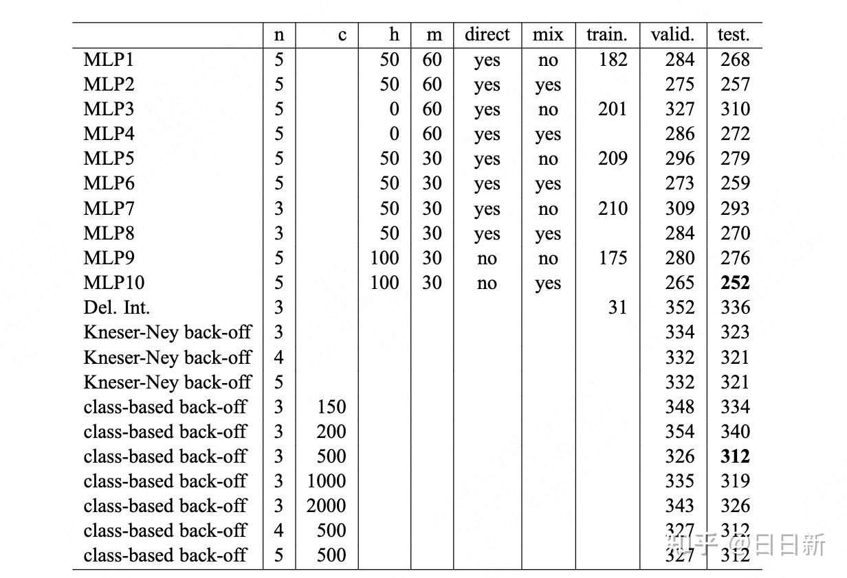
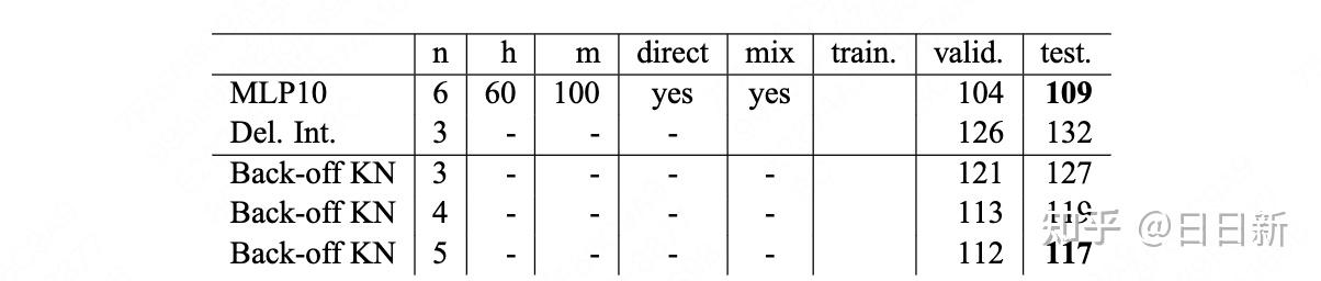


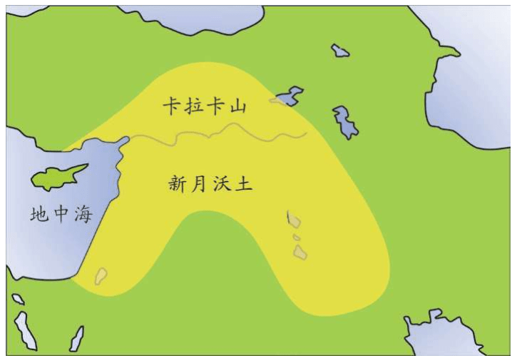
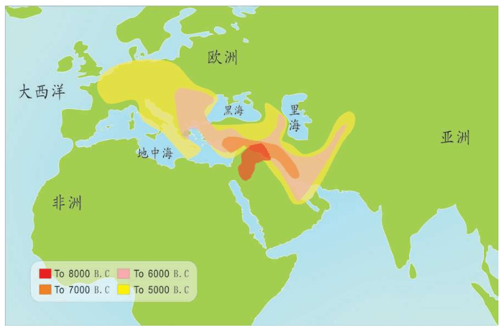
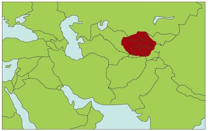
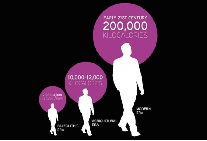
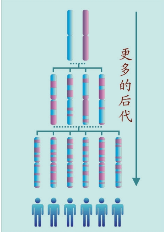
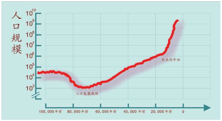
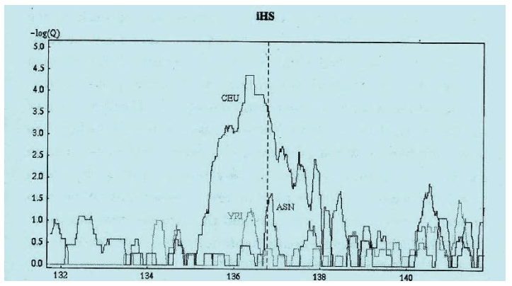
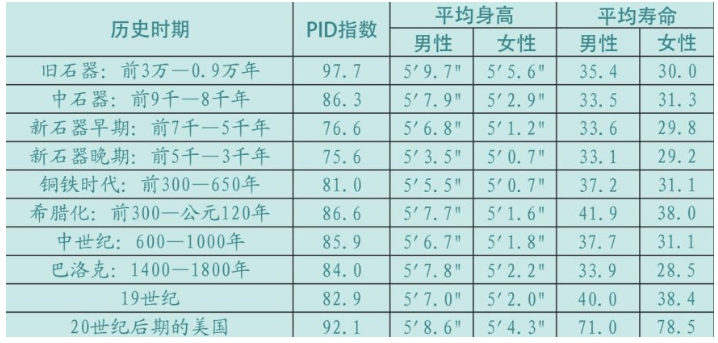
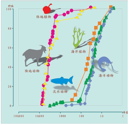
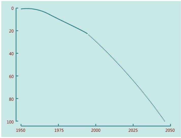
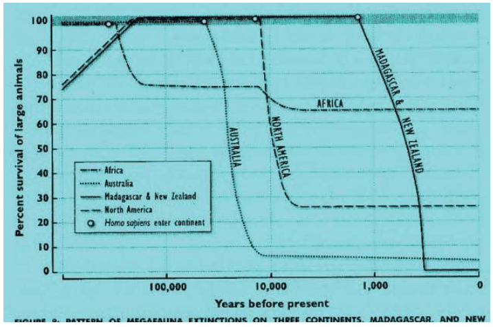
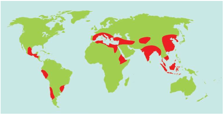
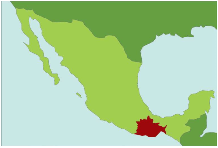

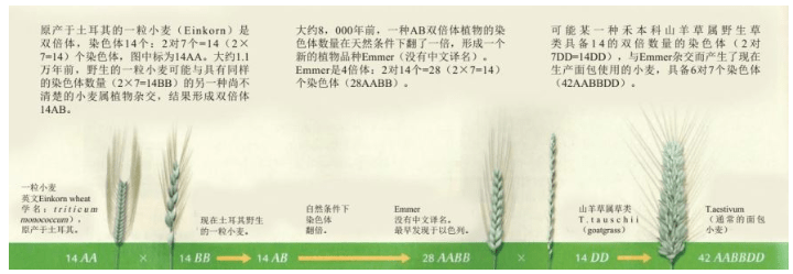
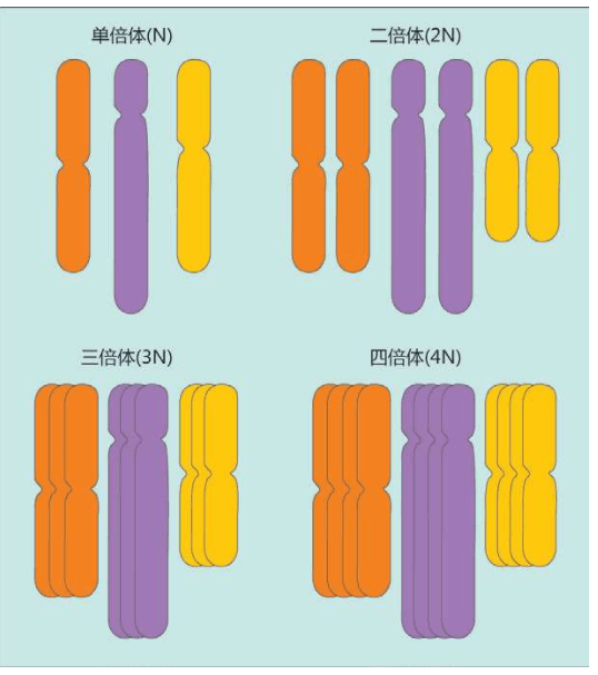
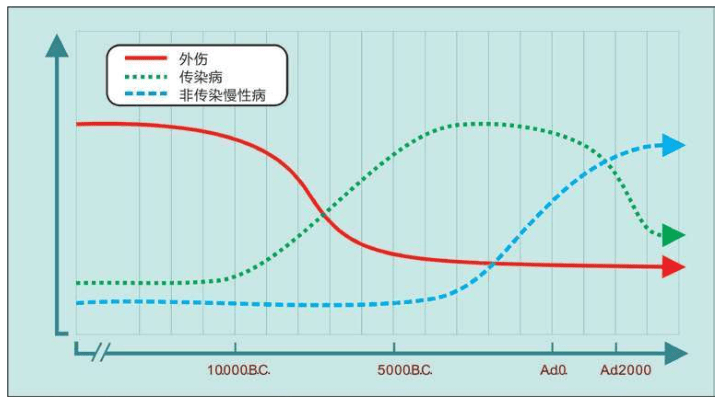
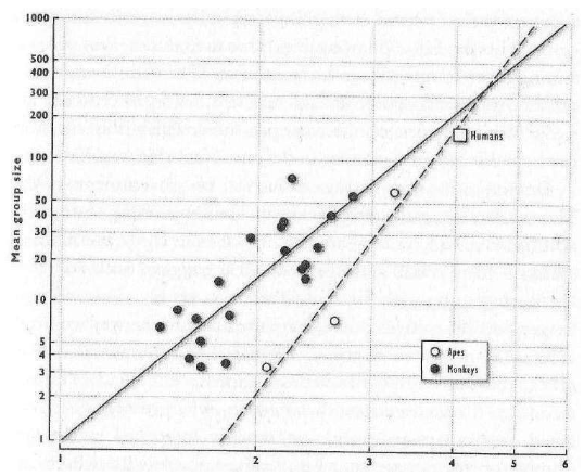
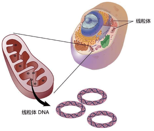
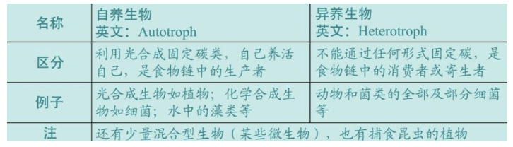
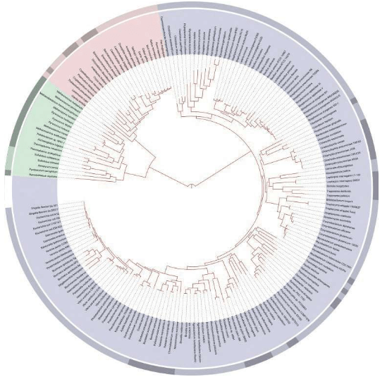
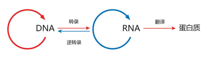
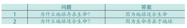
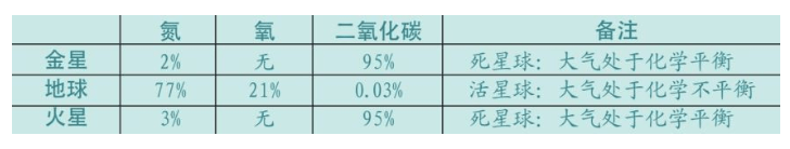
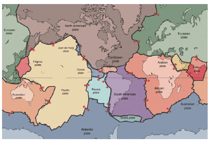
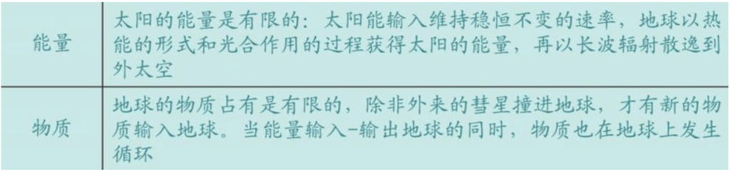
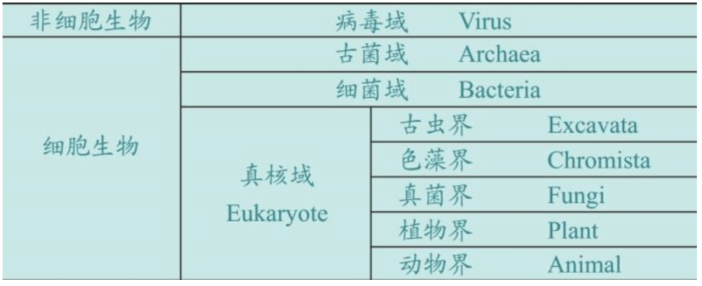
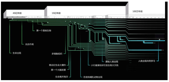
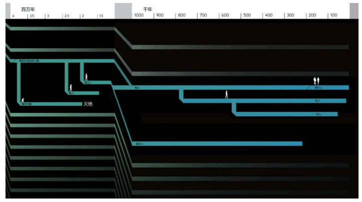
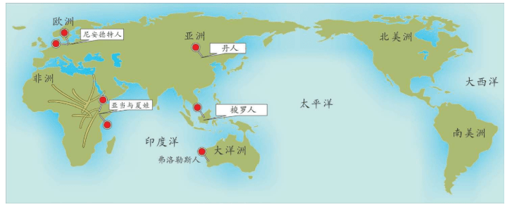
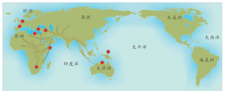
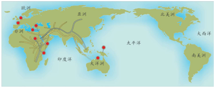
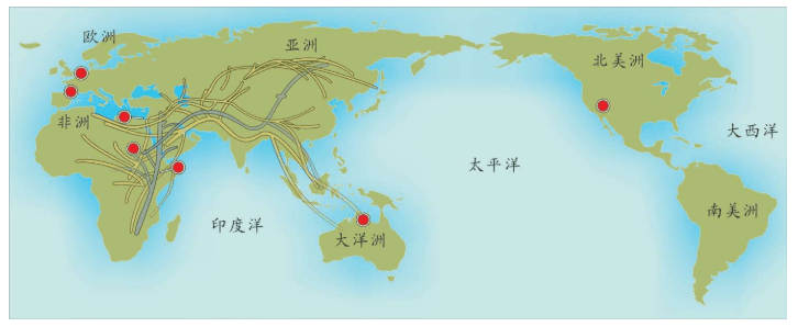
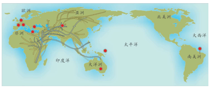
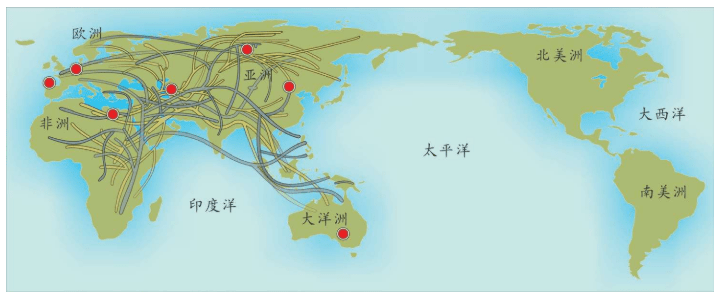
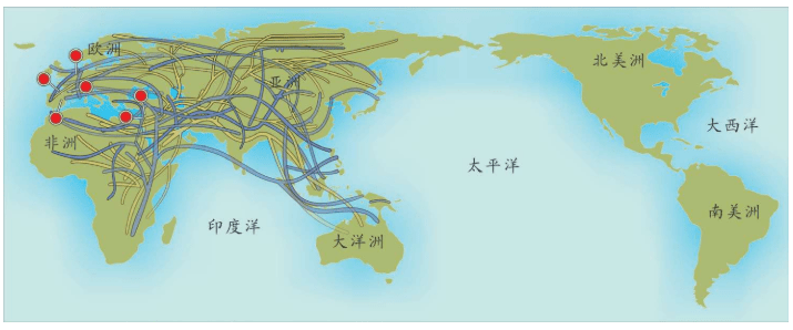
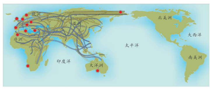
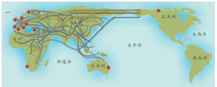
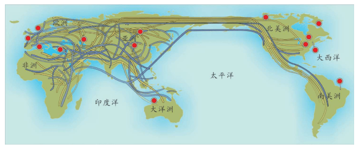
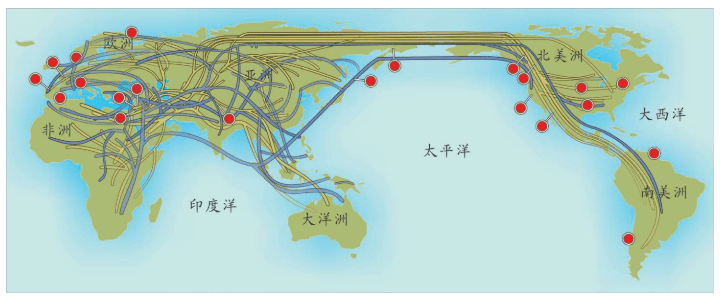
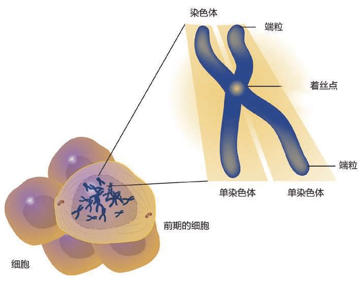
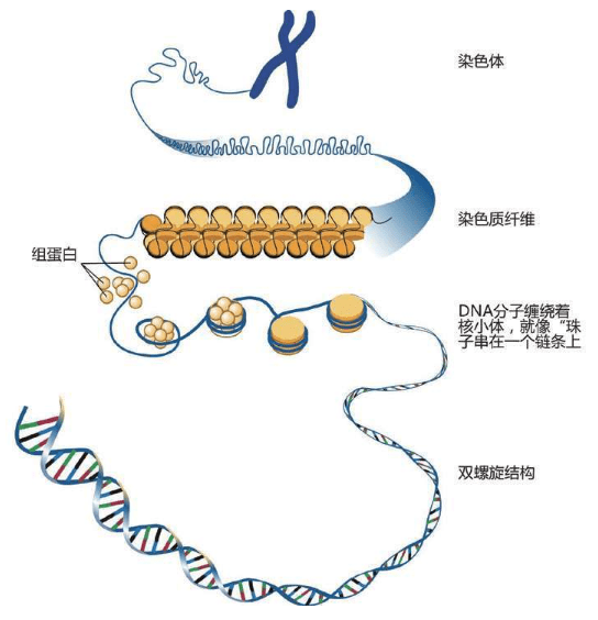
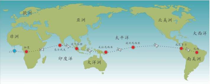
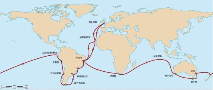
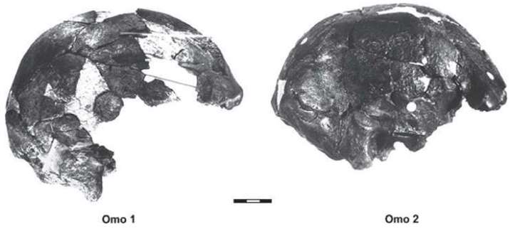
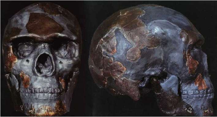
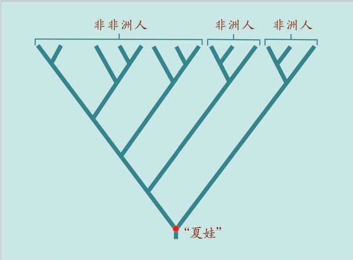
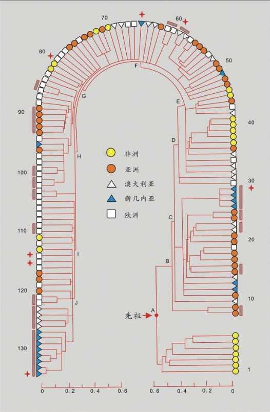
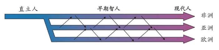
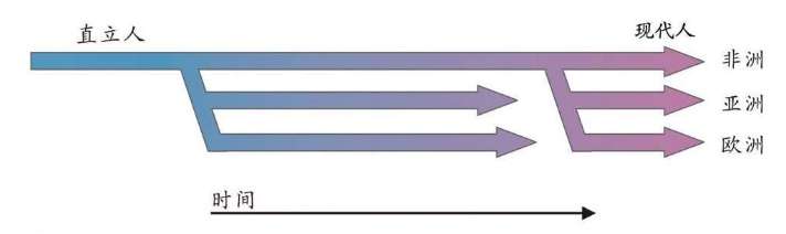
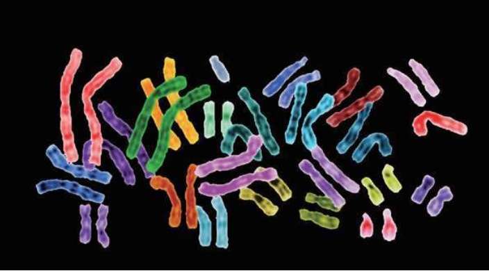
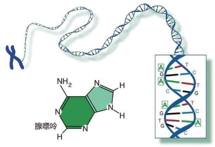
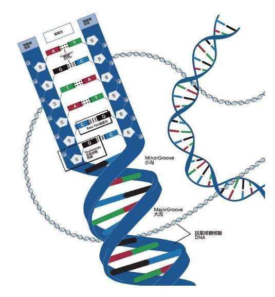
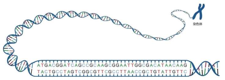
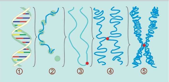
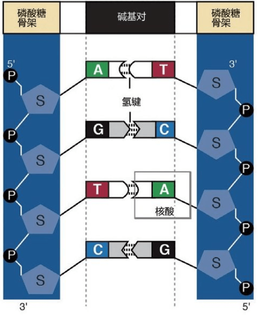
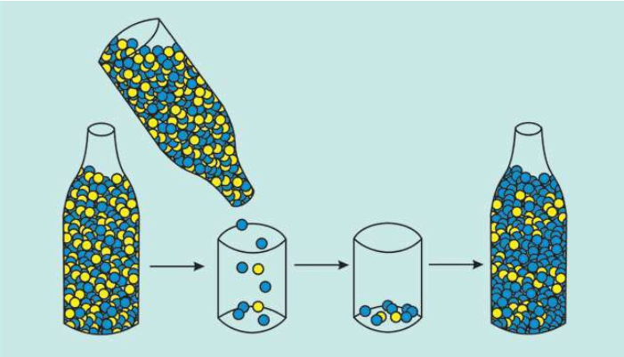
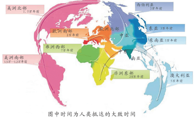
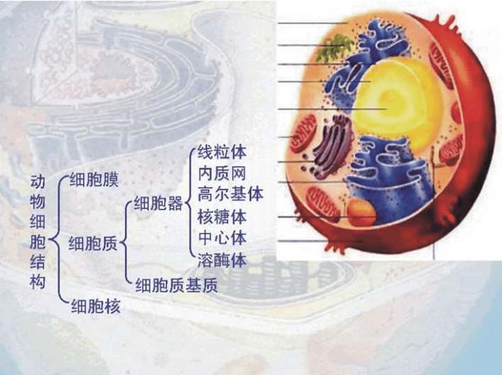
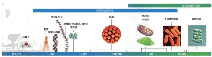
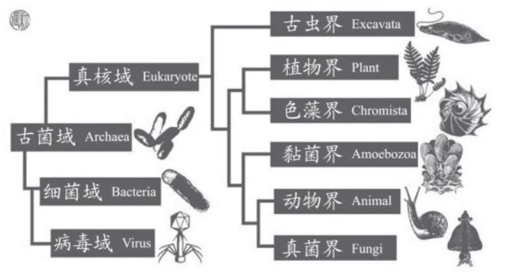
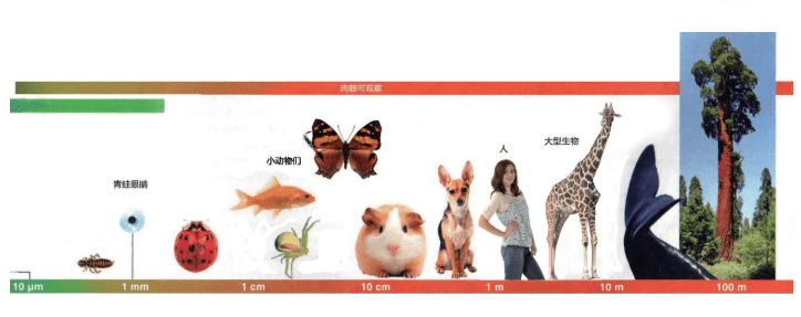
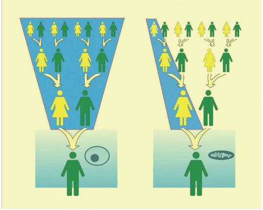
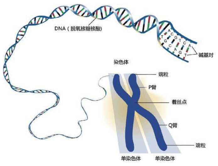
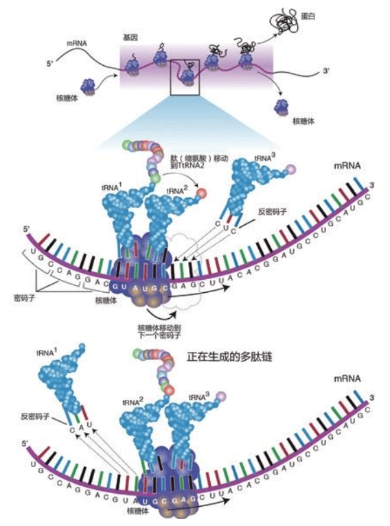
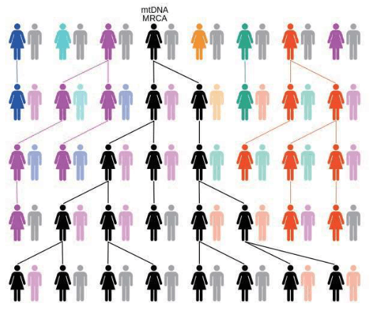
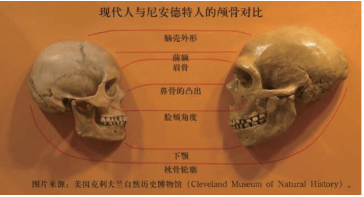
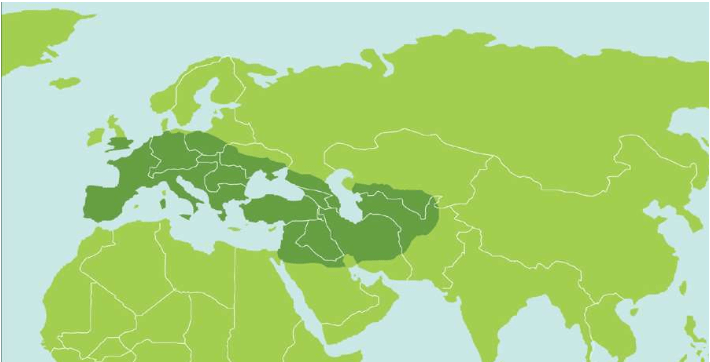
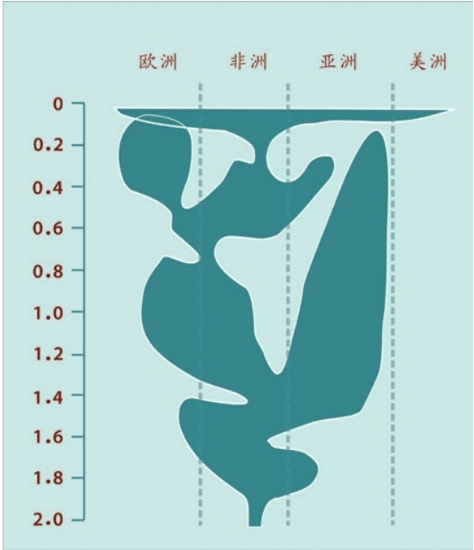

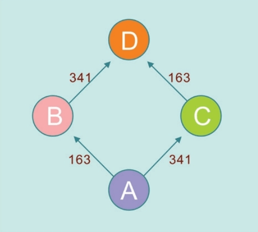
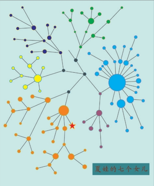
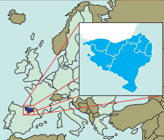
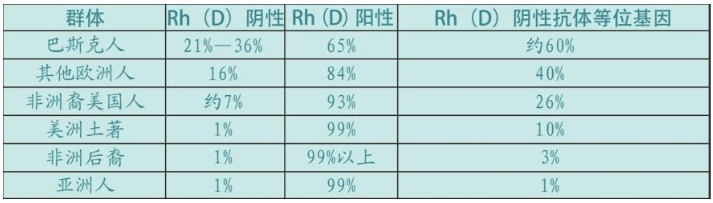
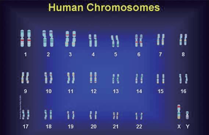
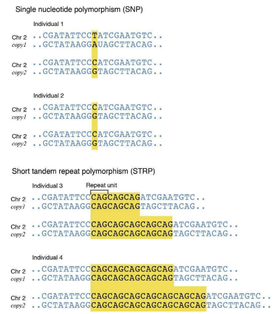
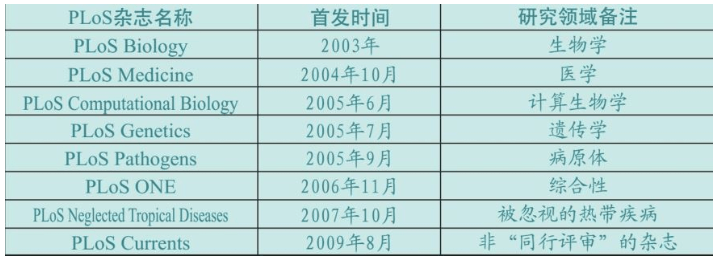
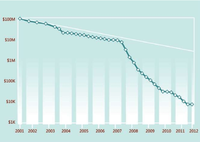
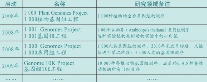
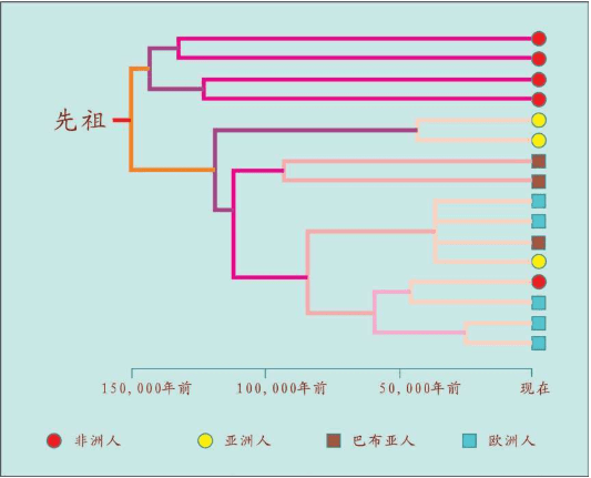
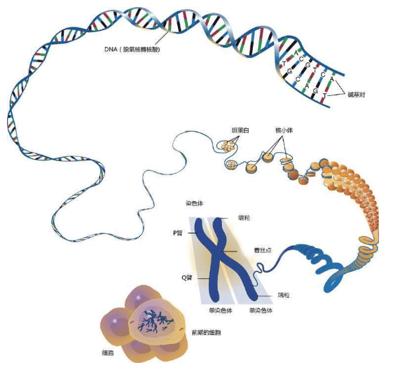
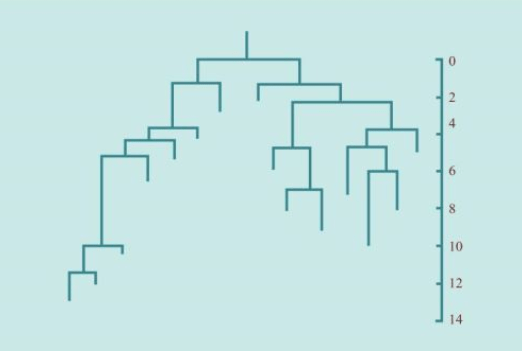
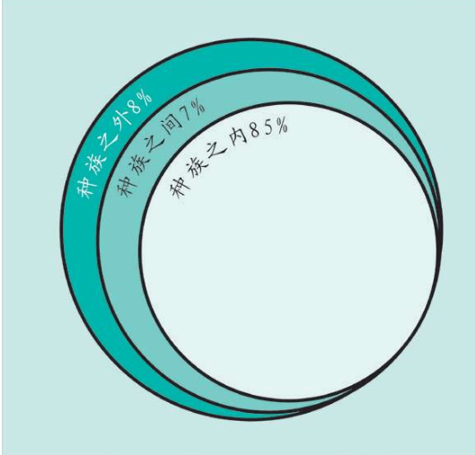
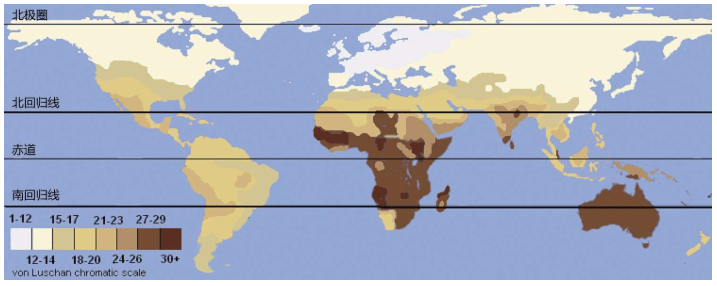
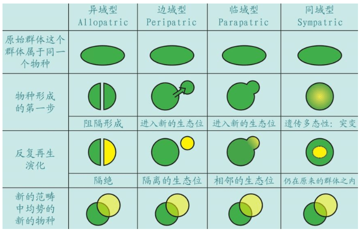
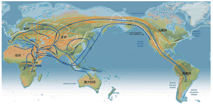
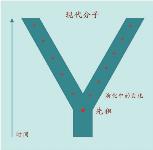
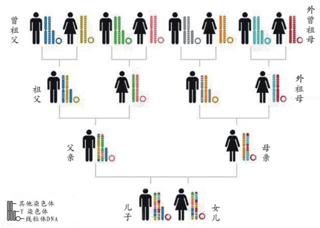
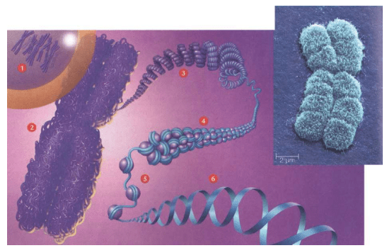
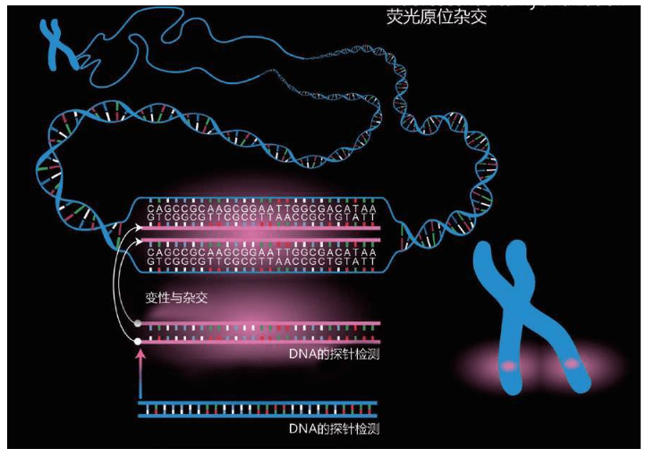
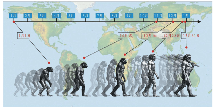
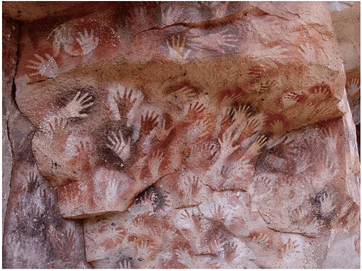
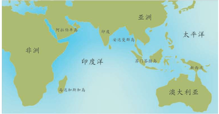
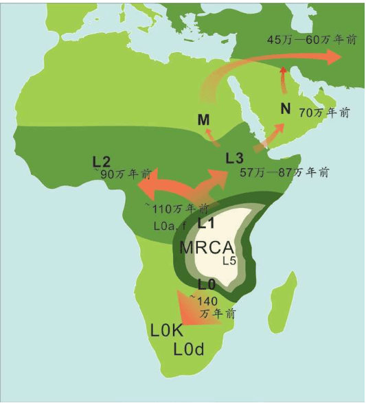
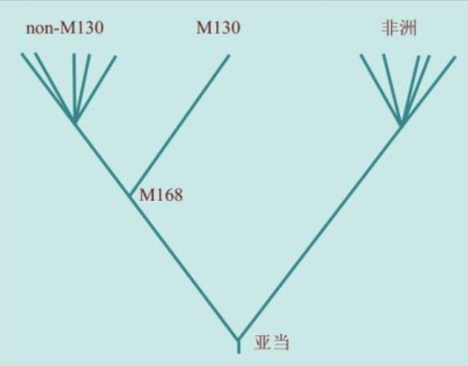
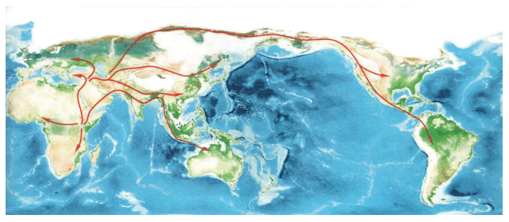
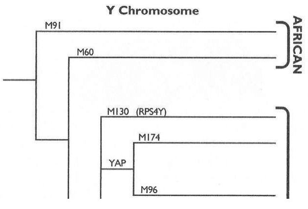
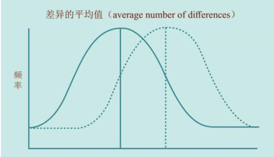
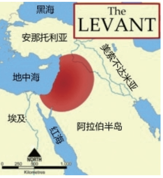
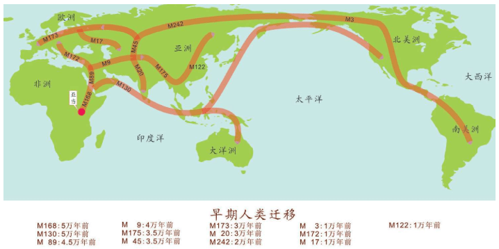
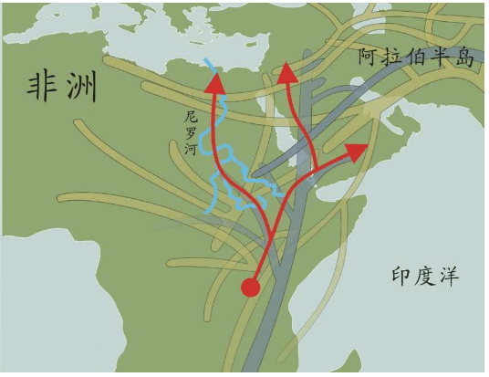
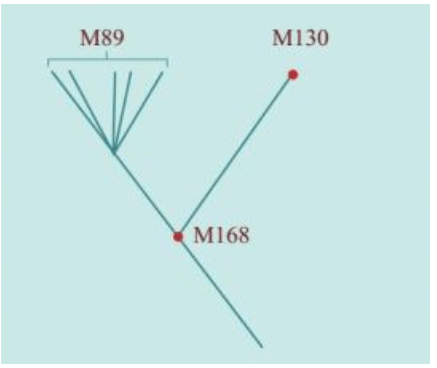
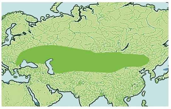
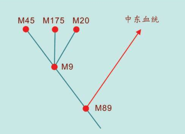
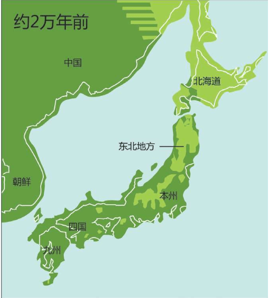
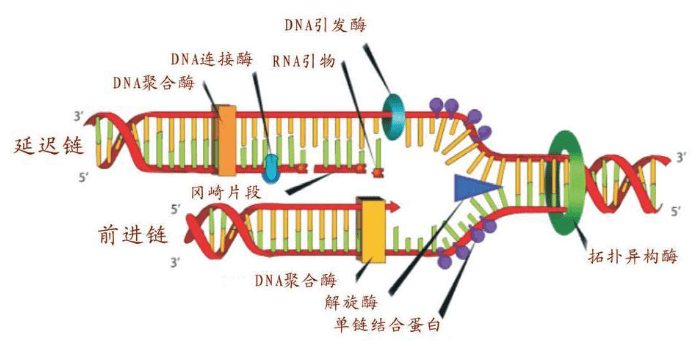
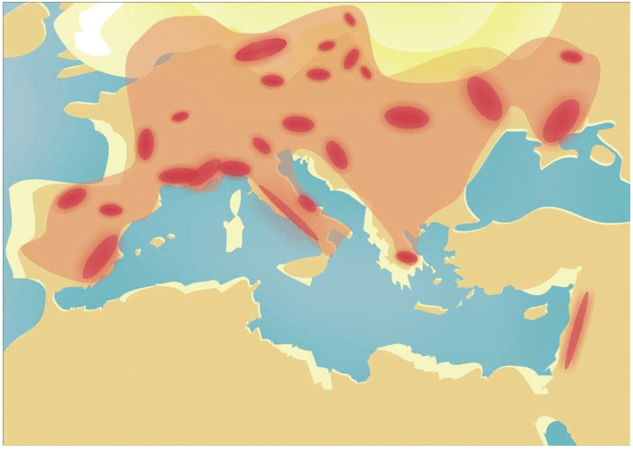
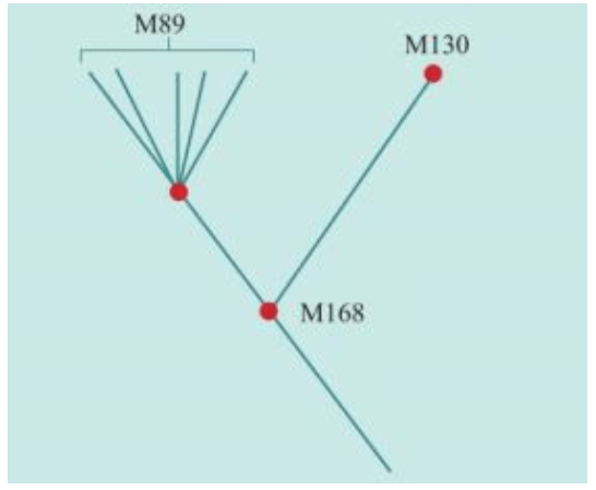
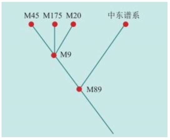
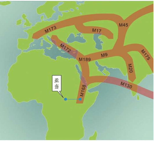
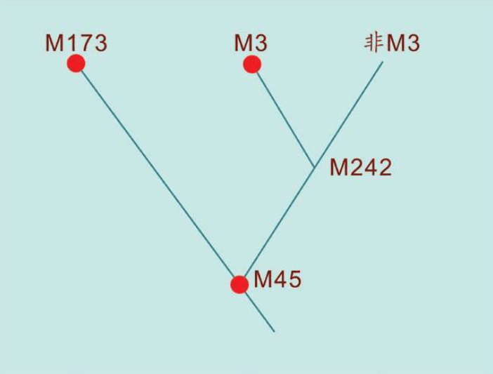
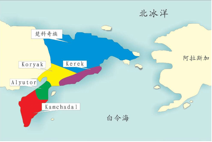
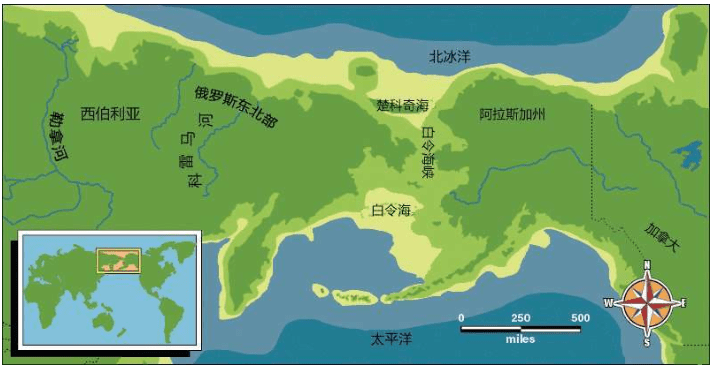
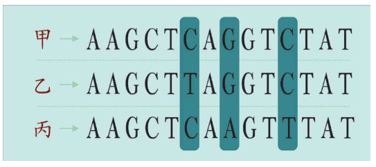
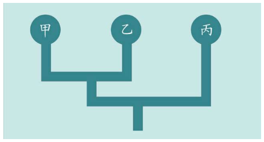
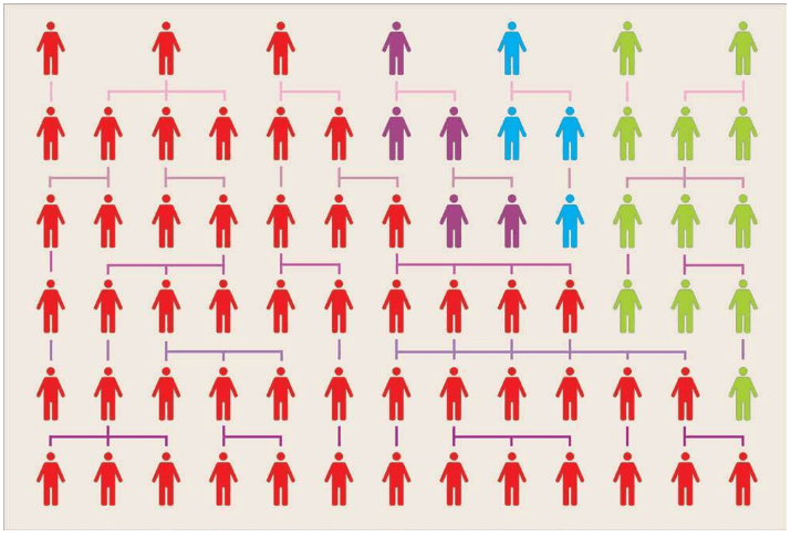
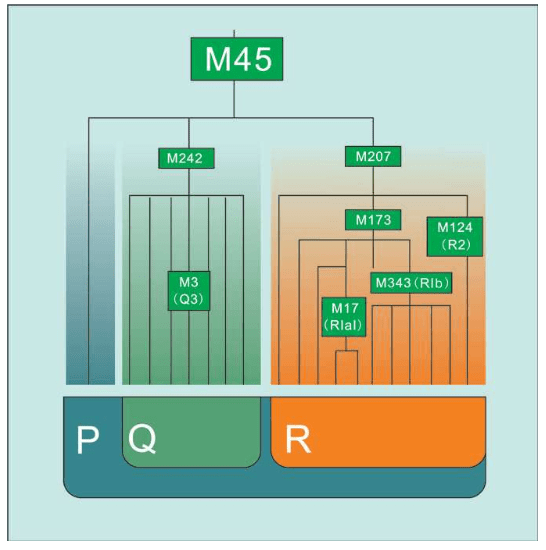
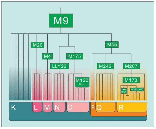
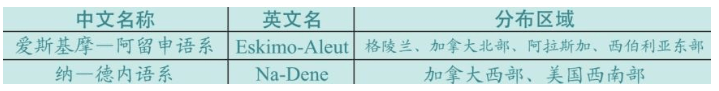
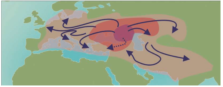
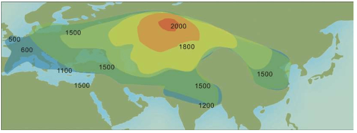
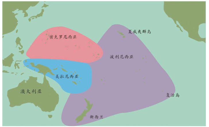
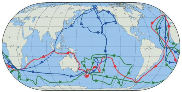
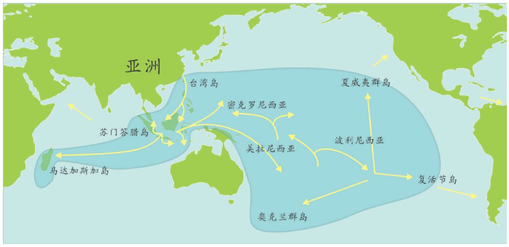
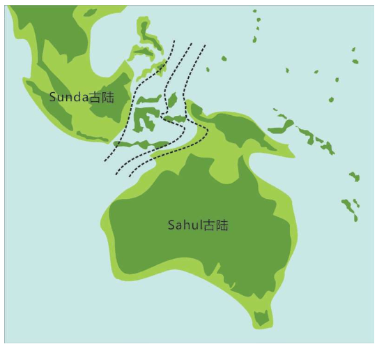
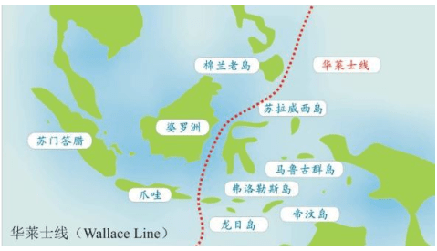
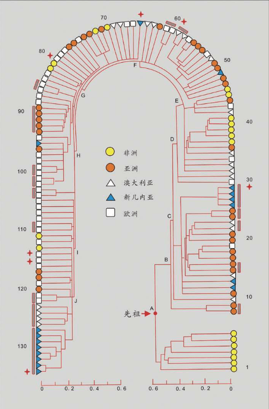
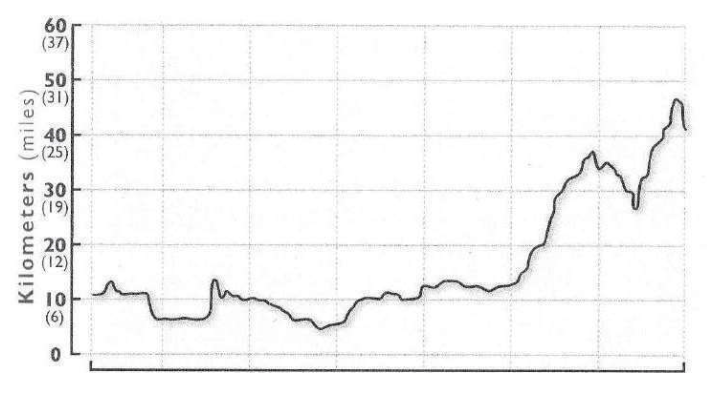
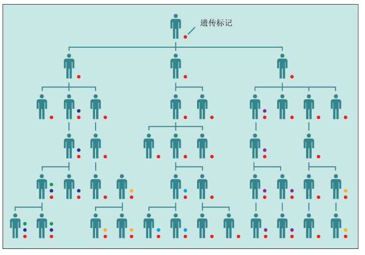
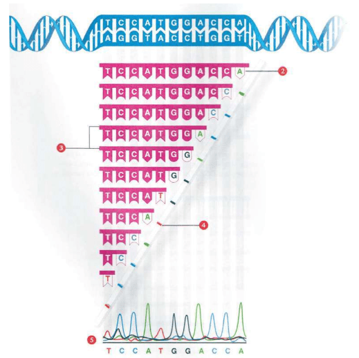
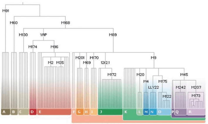
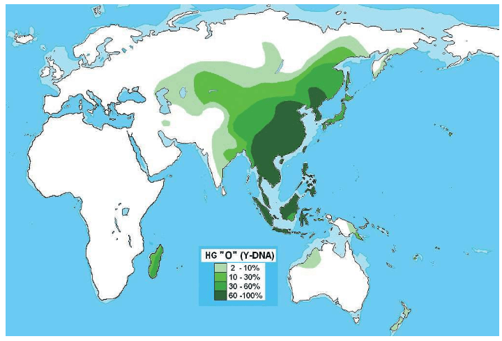
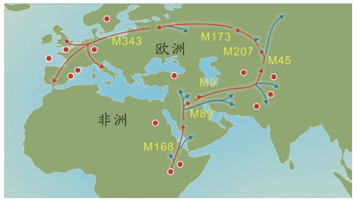
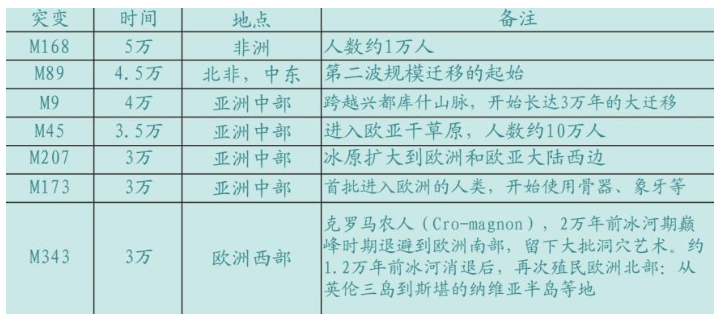
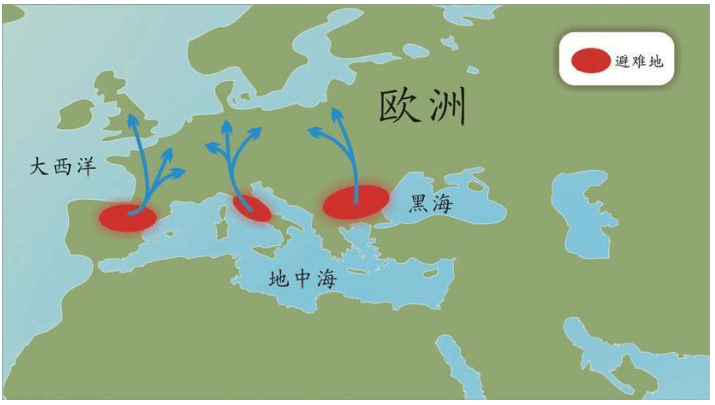
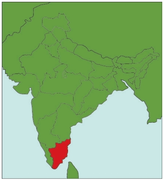
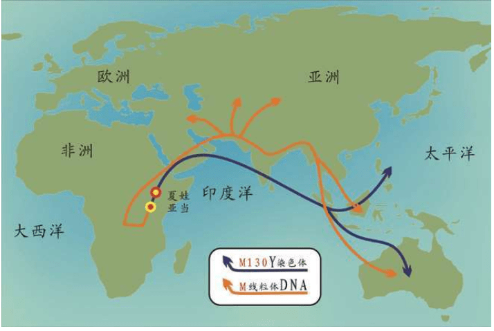
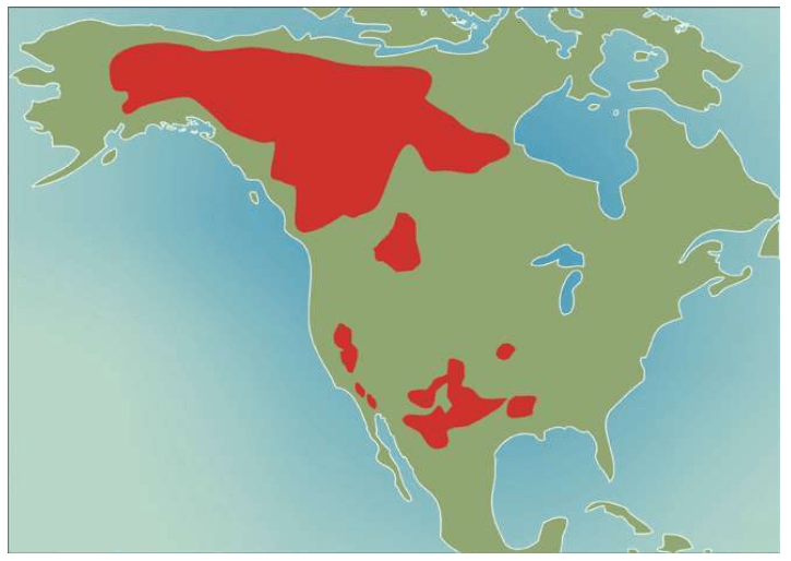
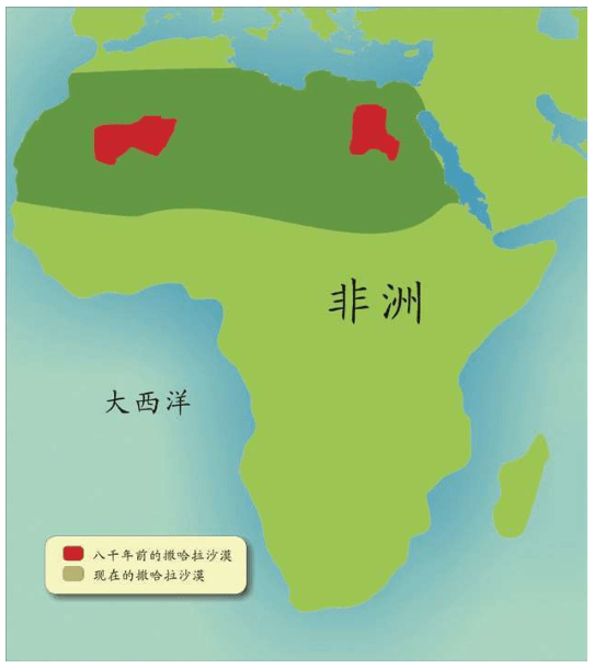
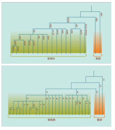
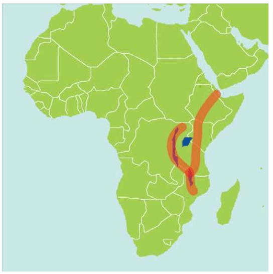
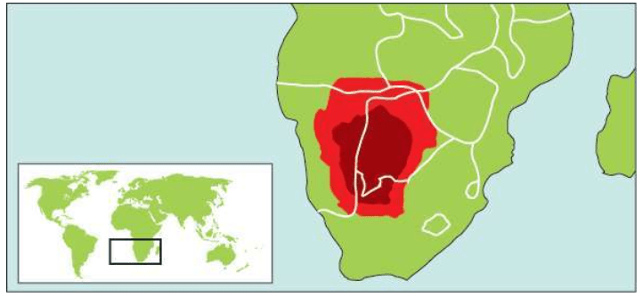
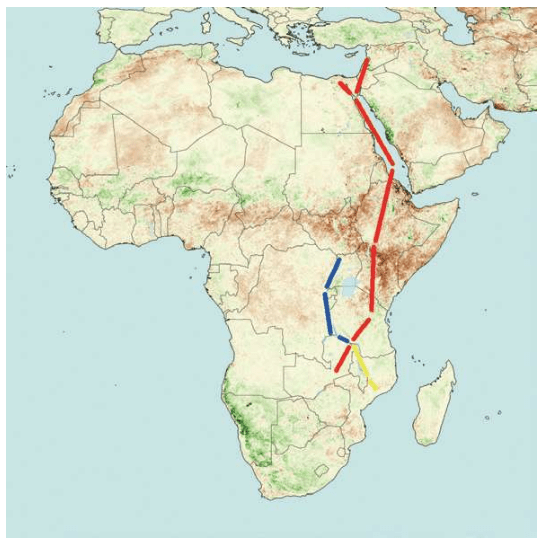
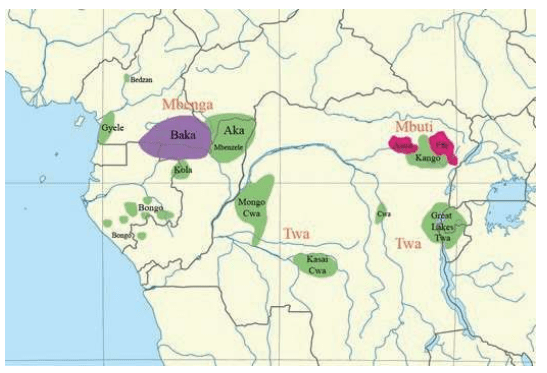
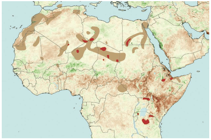
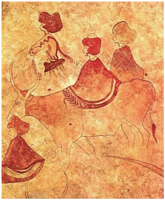


 比
比 铭记道:“其邑彶眔句、商、儿,眔雠、找,
 (复)限余(予)
 比田,其邑竞、
 (槌)、甲三邑,州、泸二邑,凡复友(贿)、复付
 比田十又三邑。”(04466)上述诸邑均有名称,在领属关系调整时作为基本单位。以邑为分封基本单位之例,如宜侯夨簋铭文记周王将虎侯夨改封于宜,有“厥川三百……厥……百又……厥宅邑卅又五,〔厥〕……百又
 ”。“厥宅邑卅又五”,当是宜城之外35邑。春秋时期齐子仲姜镈铭文也记齐侯“赐之邑,二百又九十又九邑”。这都是十分明确地将邑作为分封单位之例。
 (社)
(社)
 ,宫地主一
,宫地主一 ”,同“社”。《说文》:“
 ,古文社。”“野地主”“宫地主”“地主”则为社的别称。周家台简牍《日书》中也有田社、里社的记载。如《三十六年置居》载:
 、木并主岁。
 、冢主岁,岁为上。
 ,同“
,同“ ”,即“社”。可见,祈年是祭社的重要诉求,祈求的是“岁为上”。清华大学藏战国简《祷辞》也载有“邑又(有)社而向(乡)又(有)
  (丘)”,明确表明战国村落居民之社祭。
 ,率以春秋之月。
 (拜),言曰:“人皆祠泰父,我独祠先农。”到囷下,为一席,东乡 (向),三腏,以酒沃,祝曰:“某以壶露、牛胙,为先农除舍。先农笱(苟)令某禾多一邑,先农
  (恒)先泰父食。”
 案”案宗中,可以看到其组织方式。简文中的
 为大夫沛之妾,沛妻死后,大夫沛欲以
 所四人,不取(娶)妻矣。欲令
 (饮)食。 快等曰:可。
  即入宗,里人不幸死者出单赋,如它人妻。


